Skip Zero in Graph

[rahulbassi268]

Hello All,

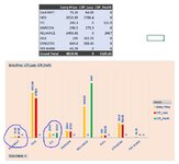
I am using Pivot Graph. In the pivot table, I had 2 columns: Entry Price & Current Price. The Bar was looking fine. But, I wanted to have Red bars for trades in Loss and Green for those in Profit.
So, for this, I added 2 calculated fields: LTP_Loss and LTP_Profit and hide that Current Price field as I no longer needed to display it.

I got the Red & Green color bars for Loss & Profit, but the zero is creating Problem.
The Zero is appearing as Gap and also as label hanging in the chart area...

My Calculated fields are as follows:
LTP_Loss = IF('Total Average Cost'>'Current Price','Current Price',0)
LTP_Profit = = IF('Current Price' >='Total Average Cost','Current Price',0)

I tried having space instead of Zero in the Else part of these formulae, but then the formulae return #Value

Please suggest.

Thanks.
Rahul

 

[rahulbassi268]

Hello All,

I was able to resolve this by simply changing the formatting of two columns in Pivot table to: 0;-0;;@
This way, these columns will display all data but zero.
So, in graph, those bars with zero are skipped.

Thanks
Rahul

 

[Peter_SSs]

My Calculated fields are as follows:
LTP_Loss = IF('Total Average Cost'>'Current Price','Current Price',0)
LTP_Profit = = IF('Current Price' >='Total Average Cost','Current Price',0)

I tried having space instead of Zero in the Else part of these formulae, but then the formulae return #Value

Seems like you may already have a suitable solution but instead of zero in those formula you could try

= IF('Total Average Cost'>'Current Price','Current Price',NA())

Generally with graphs, #N/A values are ignored. If that works and you don't want the visual #N/A you could conditionally format the cell(s) to hide them.

 

[rahulbassi268]

Seems like you may already have a suitable solution but instead of zero in those formula you could try

= IF('Total Average Cost'>'Current Price','Current Price',NA())

Generally with graphs, #N/A values are ignored. If that works and you don't want the visual #N/A you could conditionally format the cell(s) to hide them.

Hello Peter,

Thanks for your suggestion. I tried modifying my formula to below for 1 field:

LTP_Loss = IF('Total Average Cost'>'Current Price','Current Price',NA())

The table and graph starting displaying #NA.

So, I changed the option in Pivot options ("For error Values Show" checkbox). Then, the table started to hide #NA, but the graph still displayed zero.

Thanks
Rahul