=SMALL(CHOOSE SIMPLIFY

[Mjkqb]

I'm an Excel novice.

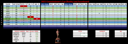
For "PUTTS", "FAIRWAYS" and "GIR" using ex: =SMALL(CHOOSE({1,2,3,4,5,6,7,8,9,10,11},D3,D4,D5,D6,D7,D8,D9,D10,D11,D12,D13),1) =SMALL(CHOOSE({1,2,3,4,5,6,7,8,9,10,11},D3,D4,D5,D6,D7,D8,D9,D10,D11,D12,D13),2)
=SMALL(CHOOSE({1,2,3,4,5,6,7,8,9,10,11},D3,D4,D5,D6,D7,D8,D9,D10,D11,D12,D13),3)

This brings down three leaders from columns "Putts - TL", "FW - TL" and "GIR - TL"
First of all is there a simpler code? This is the only way I could make it work.
I would like to bring down the players name in the adjacent cell.
I know you'll need additional info. Just let me know.

Thanks

 

[jasonb75]

You don't need to use CHOOSE for that, =SMALL(D3:D13,1) should be adequate.

To get the player name try =INDEX($B:$B,AGGREGATE(15,6,ROW($D$3:$D$13)/($D$3:$D$13=L16),COUNTIF(L$16:L16,L16)))

Tried counting the columns in your picture, hopefully it is close.

 

[Eric W]

Welcome to the forum!

How about:

Book1
	A	B	C	D	E	F	G	H	I	J	K	L	M	N	O	P	Q	R	S	T
1
2		Player		Putts - TL	FW - TL	GIR - TL
3		Barbee		1	23	12
4		Briden		2	20	20
5		Evans		6	21	1
6		Malloy		12	21	9
7		McCall		53	44	1
8		Norris		11	21	1
9		Nordstrom		8	50	1
10		Kennedy		5	1	60
11		Coates		7	12	1
12		E Logan		4	21	1
13		P Logan		6	18	1
14
15												Putts				Fairways			GIR
16												Barbee	1			Nordstrom	50		Kennedy	60
17												Briden	2			McCall	44		Briden	20
18												E Logan	4			Barbee	23		Barbee	12
19
Sheet12

Cell Formulas
Range	Formula
L16:M18	L16	=INDEX(SORT(B3:F13,3),{1;2;3},{1,3})
P16:Q18	P16	=INDEX(SORT(B3:F13,4,-1),{1;2;3},{1,4})
S16:T18	S16	=INDEX(SORT(B3:F13,5,-1),{1;2;3},{1,5})
Dynamic array formulas.

 

[Dave Patton]

another option to consider

N.B. You an post an extract of your spreadsheet with the forum's too XL2BB.

XLookup.xlsm
	A	B	C	D
1
2		Player	Net	Putts
3		Barbe	76	1
4		Briden	93	2
5		Evans	130	6
6		Malloy	136	12
7			140	53
8			145	11
9			147	8
10			148	5
11			148	7
12			170	4
13			174	6
14
15
16	1	Barbe	76	1
17	2	Briden	93	2
18	3	Evans	130	6
19
1d

Cell Formulas
Range	Formula
B16:B18	B16	=INDEX($B$3:$B$13,MATCH(C16,$C$3:$C$13,0))
C16:C18	C16	=SMALL($C$3:$C$13,A16)
D16:D18	D16	=XLOOKUP(B16,$B$3:$B$13,$D$3:$D$13,"",0)

 

[Mjkqb]

Wow! What a great forum. All answers were excellent.
Went with Eric W. as the simplest answer is usually the best.
I'll be back with more questions. Hopefully, one day I can answer one.

 

[Eric W]

Glad we could help! Thanks for the feedback.