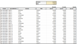
I am attempting to have the functionality to be able to filter on the [BRAND] column and receive back the summed quantity of both Types (LEGACY and NPD).
#1 - I am using the subtotal formula above each month to sum the filtered months for that particular month.
I would now like to be able to filter on other columns and receive the total of the filter for the 2 TYPES listed below.
#2 - I am using the SUMIF formula to sum the different types of data provided in the TYPE column.
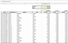
Notice that when I filter to the [CONVERSE] brand that the SUBTOTAL functionality works correctly but the SUMIF functionality does not ignore all the filtered fields as it keeps the same total even after filtering on the BRAND column.
When there may be any kind of filtering, and I want the filtered subtotals, I use a helper column that just checks if the row is visible or not (using subtotal) and then sums up the column of interest times the helper column (which is 1 or 0).
For your subtotal headers you can use the AGGREGATE function, and use the argument to ignore hidden rows.
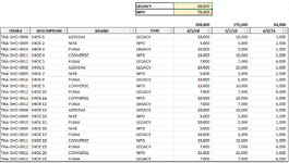
The next part I am not entirely sure if your asking for filtered values in the LEGACY and NBD cells.
For the summary at the top you can use SUM function with an calculated array (entered by CNTL-SHFT-ENTR keystroke)
IF SUM does not work, replace it with SUMPRODUCT.
We have a great community of people providing Excel help here, but the hosting costs are enormous. You can help keep this site running by allowing ads on MrExcel.com.
Allow Ads at MrExcel
Which adblocker are you using?
Disable AdBlock
Follow these easy steps to disable AdBlock
1)Click on the icon in the browser’s toolbar. 2)Click on the icon in the browser’s toolbar. 2)Click on the "Pause on this site" option.
Go back
Disable AdBlock Plus
Follow these easy steps to disable AdBlock Plus
1)Click on the icon in the browser’s toolbar. 2)Click on the toggle to disable it for "mrexcel.com".
Go back
Disable uBlock Origin
Follow these easy steps to disable uBlock Origin
1)Click on the icon in the browser’s toolbar. 2)Click on the "Power" button. 3)Click on the "Refresh" button.
Go back
Disable uBlock
Follow these easy steps to disable uBlock
1)Click on the icon in the browser’s toolbar. 2)Click on the "Power" button. 3)Click on the "Refresh" button.