Sumifs with dynamic criteria range

Rhodes19

New Member
Joined
Apr 26, 2017
Messages
18
Office Version
  1. 365
Platform
  1. Windows
Hi there, feel like there might be a simple way to do this, but I'm stumped. I'm looking for a way to have a sumifs criteria range tie to a reference rather than be static. Here's an example table (image attached as well, just in case), and my problem outlined below:

Thanks for your help!
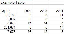
Example Table:
Sq. Ft.
2022​
2023​
2024​
85,783​
0​
8​
11​
5,837​
6​
0​
7​
6,070​
21​
44​
0​
261,674​
0​
5​
17​
7,575​
98​
12​
3​

Desired Outcome:

Create three sums of column A data, one for each year, summing only those data points that are greater than zero in the respective year

For example, 2022 should be A5+A6+A8, for a total of 19,482

Problem:

I want the formula to search within cols B-D and sum the correct year based on a reference, rather than me having to manually change the column in the formula

For example, for the 2022 total, I would want to replace the absolute reference in the below formula (B4:B8) with something dynamic
=SUMIFS(A4:A8,B4:B8,">"&0)

Also Tried:

Using IF(COUNTIF to look for a value within the range (eg 2022), but then I don't know how to tell it to do the sumifs only for the columns that contain that value
 

Attachments

  • MrExcel Table.JPG
    MrExcel Table.JPG
    18.1 KB · Views: 7

Excel Facts

Fastest way to copy a worksheet?
Hold down the Ctrl key while dragging tab for Sheet1 to the right. Excel will make a copy of the worksheet.
Rhodes Let's get the ball rolling. If this is the solutions to your problem, than good. If there are more questions than let us know.

Book1
ABCD
1Sq.Ft202220232024
285.7830811
35.837607
46.0721440
5261.6740517
67.57598123
719.482361.102360.869
Data
Cell Formulas
RangeFormula
B7:D7B7=SUMIFS($A$2:$A$6,B2:B6,">0")
 
Upvote 0
Rhodes Let's get the ball rolling. If this is the solutions to your problem, than good. If there are more questions than let us know.

Book1
ABCD
1Sq.Ft202220232024
285.7830811
35.837607
46.0721440
5261.6740517
67.57598123
719.482361.102360.869
Data
Cell Formulas
RangeFormula
B7:D7B7=SUMIFS($A$2:$A$6,B2:B6,">0")
Thanks for answering! However, that's basically the same formula I already have, and what I want to do is NOT have to hardcode B2:B6 (or C2:C6, etc). The file this comes from is more complex than this simplified example. The data output is on a different tab with a list of years, and I want to reference those cells in my formulas, as the reference years will change, though the data table will not.

Let me know if that explains it better!
 
Upvote 0
Ok Rhodes, Now I am going to assume those are the correct totals you want to see. If that is true than we can move on to your next criteria the data output is on a different tab. As you can see below, we can reference a different tab in the formula. As far as the hardcoding, if we can hold off on that until you are happy with the different tab criteria, I am sure we can solve that problem. Again this usually generates more questions than answers so, let the discussion begin.

Book1
ABCD
1Sq.Ft202220232024
285.783
35.837
46.07
5261.674
67.575
719.482361.102360.869
Data 1
Cell Formulas
RangeFormula
B7:D7B7=SUMIFS($A$2:$A$6,'Data 2'!B2:B6,">0")


Book1
ABCD
1Sq.Ft202220232024
20811
3607
421440
50517
698123
Data 2
 
Upvote 0
See if either of these options are of interest.

BTW, I suggest that you investigate XL2BB for providing sample data to make it easier for helpers by not having to manually type out sample data to test with.

23 07 29.xlsm
ABCDEFGHI
1Totals
2202220232024202220232024
35000081114000216000215000
4300060714000216000215000
5400021440
62000000517
7700098123
Yearly Sums
Cell Formulas
RangeFormula
G3:I3G3=SUMIFS($A3:$A7,INDEX($B3:$D7,0,MATCH(G2,$B2:$D2,0)),">0")
G4:I4G4=SUM(FILTER($A3:$A7,FILTER($B3:$D7,$B2:$D2=G2)>0))
 
Upvote 0

Forum statistics

Threads
1,215,069
Messages
6,122,956
Members
449,096
Latest member
Anshu121

We've detected that you are using an adblocker.

We have a great community of people providing Excel help here, but the hosting costs are enormous. You can help keep this site running by allowing ads on MrExcel.com.
Allow Ads at MrExcel

Which adblocker are you using?

Disable AdBlock

Follow these easy steps to disable AdBlock

1)Click on the icon in the browser’s toolbar.
2)Click on the icon in the browser’s toolbar.
2)Click on the "Pause on this site" option.
Go back

Disable AdBlock Plus

Follow these easy steps to disable AdBlock Plus

1)Click on the icon in the browser’s toolbar.
2)Click on the toggle to disable it for "mrexcel.com".
Go back

Disable uBlock Origin

Follow these easy steps to disable uBlock Origin

1)Click on the icon in the browser’s toolbar.
2)Click on the "Power" button.
3)Click on the "Refresh" button.
Go back

Disable uBlock

Follow these easy steps to disable uBlock

1)Click on the icon in the browser’s toolbar.
2)Click on the "Power" button.
3)Click on the "Refresh" button.
Go back
Back
Top