SUMPRODUCT multiple criteria

[mikemathis]

I'm trying to modify a SUMPRODUCT formula to include a limiting criteria of a person's name.

Here's the current formula:
=IF(B5="","",SUMPRODUCT(--ISNUMBER(FIND($B5,'2024_Offering'!$B$2:$B$750))*(E1,'2024_Offering'!C2:C750)*('2024_Offering'!$A$2:$A$750>=$C$1)*('2024_Offering'!$A$2:$A$750<=$C$2),'2024_Offering'!$D$2:$D$750))

Where:
B2:B750 is "Regular Offering"
E1 would be the givers name (this added part fails the formula)
C1 is the start date
C2 is the end date
D2:D750 is the dollar amount (which I want to total)

Any help appreciated.
Mike

 

[KRice]

Try changing this
(E1,'2024_Offering'!C2:C750)
to this
('2024_Offering'!$C$2:$C$750=$E$1)
and you may want to make the reference to E1 fixed rather than relative.

You can also eliminate the double unary (—) since the multiplication of that array with other arrays will automatically corerce TRUEs to 1 and FALSEs to 0.

 

[mikemathis]

KRice. That is the 'ticket'. Thanks much. I wish I could say I fully understand the formula, but it does precisely what I need.

many thanks.
Mike

 

[KRice]

Glad to help. About the formula, the messiest part involves the SUMPRODUCT function. In it, you are essentially creating four arrays using logical checks, each array indicating which rows satisfy one particular condition:

ISNUMBER(FIND($B5,'2024_Offering'!$B$2:$B$750)) ...searches for the text in B5 in the range '2024_Offering'!$B$2:$B$750 and returns a number indicating the character position where the match occurs on each row; and if no match is found, then a #VALUE! error is created. So this gives an array of 749 elements (the row range runs from 2 to 750, which is 749 elements) that are either a number or a #VALUE! error. The numbers are indicative of a match, so those rows need to be considered (and used if all other criteria are met). To convert this 749 element array to something more useful, it is operated on by the ISNUMBER function to return either TRUE where an array element is a number or a FALSE everywhere else, including the errors.

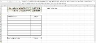
('2024_Offering'!$C$2:$C$750=$E$1) ...creates a 749 element array indicating which cells in '2024_Offering'!$C$2:$C$750 match the name in $E$1, and each element is either TRUE or FALSE

('2024_Offering'!$A$2:$A$750>=$C$1) ...creates a 749 element array indicating which cells in '2024_Offering'!$A$2:$A$750 contain dates that occur on or after the "From" date in $C$1, and each element is either TRUE or FALSE

('2024_Offering'!$A$2:$A$750<=$C$2) ...creates a 749 element array indicating which cells in '2024_Offering'!$A$2:$A$750 contain dates that occur on or before the "To" date in $C$2, and each element is either TRUE or FALSE

When these arrays are multiplied together, the result is a single 749 element array. The arithmetic operation (multiplication in this case since you want all four conditions to be true simultaneously) will automatically coerce any TRUEs to assume a value of 1, and any FALSEs to assume a value of 0. So the end result is an array of 1's and 0's.

Then the SUMPRODUCT function reduces to something like this:
SUMPRODUCT( {resultant array of 1's and 0's}, '2024_Offering'!$D$2:$D$750 )
...which multiples each item in '2024_Offering'!$D$2:$D$750 by either 0 (representing rows where at least one condition is not satisfied) or 1 (representing rows where all conditions are satisfied).