Tiered Calculation Formula

jayjay123

New Member
Joined
Jun 3, 2021
Messages
45
Office Version
  1. 365
Platform
  1. Windows
Hi there,

Would someone be able to help me build a formula that will calculate the total $ value according to the appropriate tier.

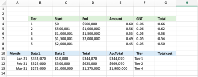
The first extract 1 is a tier structure table. Between certain values, a set pricing will be applicable. e.g. values between $0 - $100,000 will be Tier 1 at the rate of $0.66 cents.
In extract 2, we have the monthly total in column A, and a cumulative YTD in column B. Column 3 - categorises these in the appropriate tier.


Can you please help me design an excel formula to calculate column D?
Extract 2:
- Tier 2 - Calculation should be $165,000.
- First $100,000 @ $0.66 = $66,000
- Remaining $65,000 @ $0.63 = $40,950
Total should be: $106,950

Extract 1:

TierStartEnd$
1$0.00$100,000.000.66
2$100,000.01$250,000.000.63
3$250,000.01$500,000.000.55
4$500,000.01$999,999.000.50


Extract 2:
Month totalCumulative YTDValueCalculation
$40,000.00$40,000.00Tier 1
$125,000.00$165,000.00Tier 2
$275,000.00$400,000.00Tier 3
$540,000.00$815,000.00Tier 4

Thanks very much for your help
 

Excel Facts

Can you AutoAverage in Excel?
There is a drop-down next to the AutoSum symbol. Open the drop-down to choose AVERAGE, COUNT, MAX, or MIN
C2 I named the array of Bracket data aB {0;100000;250000;500000} and
I named the array of Rate Differentials aR {0.66;-0.03;-0.08;-0.05
With the named arrays, we do not need the table of Brackets / Tiers.

Commissions 2021.xlsm
ABCD
1Total sales165,000.00
2Commission106,950.00106,950.00
3Commission Arithmetic106,950.00
4
5The Table below is not required.
6BracketsRates
7
8066%66,000.0066,000.00
9100,00063%40,950.00106,950.00
10250,00055%106,950.00
11500,00050%106,950.00
121E+308
1c
Cell Formulas
RangeFormula
C2C2=SUMPRODUCT(--(B1>aB),B1-aB,{0.66;-0.03;-0.08;-0.05})
B2B2=SUMPRODUCT(--(B1>A8:A11),B1-A8:A11,B8:B11-B7:B10)
B3B3=MAX(D8:D11)
C8:C9C8=MAX(0,MIN($B$1,A9)-A8)*B8
D8:D11D8=MAX(0,MIN($B$1,A9)-A8)*B8+D7
B12B12=BigNum
 
Last edited:
Upvote 0
Commissions 2021.xlsm
ABCD
1Total sales815,000.00
2Commission455,500.00455,500.00
3Commission Arithmetic455,500.00455,500.00
4
5The Table below is not required.
6BracketsRates
7
8066%66,000.0066,000.00
9100,00063%94,500.00160,500.00
10250,00055%137,500.00298,000.00
11500,00050%157,500.00455,500.00
121E+308
1c
Cell Formulas
RangeFormula
B2B2=SUMPRODUCT(--(B1>A8:A11),B1-A8:A11,B8:B11-B7:B10)
C2C2=SUMPRODUCT(--(B1>aB),B1-aB,{0.66;-0.03;-0.08;-0.05})
B3B3=MAX(D8:D11)
C3C3=SUM(C8:C11)
C8:C11C8=MAX(0,MIN($B$1,A9)-A8)*B8
D8:D11D8=MAX(0,MIN($B$1,A9)-A8)*B8+D7
B12B12=BigNum
 
Upvote 0
Thank you very much Dave.
I would like to keep the existing table & format as this template is used by other members of my team.
Is it possible to still make a formula?
 
Upvote 0
Hi, I had a similar problem trying to calculate progressive tax scales.
It turns out the Vlookup function can do this.

If your table [tax_table} is :

lower boundUpper boundmarginal rateBase
018,2000.000$0
18,20145,0000.190$0
45,001120,0000.325$5,092
120,001180,0000.370$29,467
180,001999,999,9990.450$51,667


The total tax payable is based on the value of the cell B4 =VLOOKUP($B$4,Tax_Table,4,TRUE)+($B$4-VLOOKUP($B$4,Tax_Table,1,TRUE)+1)*VLOOKUP($B$4,Tax_Table,3,TRUE)
NOte - I have an added column here that you do not show above - called base - this is the value of all the rows above and is used to avoid calcualting each row each ever time.

With only small changes, will solve the problem.
 
Upvote 0
Hi Kieran and Dave.

Thank you so much for your help.
I'm not very good with excel, so I'm still having a bit of trouble trying to get the right calculation even though I tried the above.

I've attached a screenshot below which might be able to help explain what I'm looking for.
I am trying to find a formula to calculate G11 onwards.
For example: Feb21 - Accumulated Total $969,070 will be made up of two pricing structures (Tier 1 + 2).

Kindly assist!
 

Attachments

  • Screen Shot 2021-06-04 at 6.04.34 pm.png
    Screen Shot 2021-06-04 at 6.04.34 pm.png
    39.1 KB · Views: 53
Upvote 0
What results do you calculate with your example?

I named the array of Bracket data aB {0;500000;1000000;1500000;2000000} and
I named the array of Rate Differentials aR {0.66;-0.04;-0.04;-0.04;-0.04}
Use Name Manager and then try the formula.

Commissions 2021.xlsm
ABCDEF
10MonthTotal
11Jan-21344,070227,086.20
12Feb-21969,070620,823.40
13Mar-211,900,0001,146,000.00
14
1d
Cell Formulas
RangeFormula
F11:F13F11=SUMPRODUCT(--(E11>aB),E11-aB,aR)
 
Upvote 0

Forum statistics

Threads
1,215,053
Messages
6,122,882
Members
449,097
Latest member
dbomb1414

We've detected that you are using an adblocker.

We have a great community of people providing Excel help here, but the hosting costs are enormous. You can help keep this site running by allowing ads on MrExcel.com.
Allow Ads at MrExcel

Which adblocker are you using?

Disable AdBlock

Follow these easy steps to disable AdBlock

1)Click on the icon in the browser’s toolbar.
2)Click on the icon in the browser’s toolbar.
2)Click on the "Pause on this site" option.
Go back

Disable AdBlock Plus

Follow these easy steps to disable AdBlock Plus

1)Click on the icon in the browser’s toolbar.
2)Click on the toggle to disable it for "mrexcel.com".
Go back

Disable uBlock Origin

Follow these easy steps to disable uBlock Origin

1)Click on the icon in the browser’s toolbar.
2)Click on the "Power" button.
3)Click on the "Refresh" button.
Go back

Disable uBlock

Follow these easy steps to disable uBlock

1)Click on the icon in the browser’s toolbar.
2)Click on the "Power" button.
3)Click on the "Refresh" button.
Go back
Back
Top