Dearest Excel Community,
I am creating box and whisker plots in Excel 2007 by utilizing stacked column charts along with custom error bars. As I create a high volume of these charts I am attempting to automate the process to increase my efficiency.
I have tried to record a macro for the process but when I implement the macro I get an error. The problem occurs when the Macro attempts to designate the custom error bars (at least that's where I think the problem occurs).
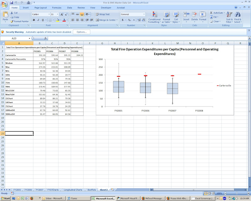
This is what my data looks like, and the chart that I am attempting to automate:
When I record my process through a Macro, here is what I get (by the way, I don't know much about VBA, but I know there's a lot of "junk" code associated with macro recording...sorry):
If anyone out there can help me, I'd greatly appreciate it. Also, I recognize that I may not have provided enough information, so please let me know if there is more info you need.
Thanks,
Tom
I am creating box and whisker plots in Excel 2007 by utilizing stacked column charts along with custom error bars. As I create a high volume of these charts I am attempting to automate the process to increase my efficiency.
I have tried to record a macro for the process but when I implement the macro I get an error. The problem occurs when the Macro attempts to designate the custom error bars (at least that's where I think the problem occurs).
This is what my data looks like, and the chart that I am attempting to automate:
When I record my process through a Macro, here is what I get (by the way, I don't know much about VBA, but I know there's a lot of "junk" code associated with macro recording...sorry):
Code:
Sub BoxPlotNew()
'
' BoxPlotNew Macro
'

'
    ActiveSheet.Shapes.AddChart.Select
    ActiveChart.SetSourceData Source:=Range("Sheet3!$B$2:$E$2,Sheet3!$B$14:$E$16" _
        )
    ActiveChart.ApplyChartTemplate ( _
        "C:\Users\tquist\AppData\Roaming\Microsoft\Templates\Charts\Whisker Chart.crtx" _
        )
    ActiveChart.SeriesCollection(1).Select
    ActiveChart.SeriesCollection(1).HasErrorBars = True
    ActiveSheet.ChartObjects("Chart 2").Activate
    ActiveChart.SeriesCollection(1).ErrorBars.Select
    ActiveChart.SeriesCollection(1).ErrorBar Direction:=xlY, Include:= _
        xlMinusValues, Type:=xlFixedValue, Amount:=20
    ActiveChart.SeriesCollection(1).ErrorBar Direction:=xlY, Include:= _
        xlMinusValues, Type:=xlCustom, Amount:=0
    ActiveSheet.ChartObjects("Chart 2").Activate
    ActiveChart.SeriesCollection(1).ErrorBars.Select
    ActiveSheet.ChartObjects("Chart 2").Activate
    ActiveChart.SeriesCollection(3).Select
    ActiveChart.SeriesCollection(3).HasErrorBars = True
    ActiveSheet.ChartObjects("Chart 2").Activate
    ActiveChart.SeriesCollection(3).ErrorBars.Select
    ActiveChart.SeriesCollection(3).ErrorBar Direction:=xlY, Include:= _
        xlPlusValues, Type:=xlFixedValue, Amount:=20
    ActiveChart.SeriesCollection(3).ErrorBar Direction:=xlY, Include:= _
        xlPlusValues, Type:=xlCustom, Amount:=0
    ActiveSheet.ChartObjects("Chart 2").Activate
    ActiveChart.SeriesCollection(3).ErrorBars.Select
    ActiveSheet.ChartObjects("Chart 2").Activate
    ActiveChart.SeriesCollection(2).Select
    ActiveChart.SeriesCollection(2).HasErrorBars = True
    ActiveSheet.ChartObjects("Chart 2").Activate
    ActiveChart.SeriesCollection(2).ErrorBars.Select
    ActiveChart.SeriesCollection(2).ErrorBar Direction:=xlY, Include:=xlBoth, _
        Type:=xlCustom, Amount:=0
    ActiveSheet.ChartObjects("Chart 2").Activate
    ActiveChart.SeriesCollection(2).ErrorBars.Select
    ActiveSheet.ChartObjects("Chart 2").Activate
    ActiveChart.PlotArea.Select
    ActiveChart.SeriesCollection.NewSeries
    ActiveChart.SeriesCollection(4).Name = "=Sheet3!$A$3"
    ActiveChart.SeriesCollection(4).Values = "=Sheet3!$B$3:$E$3"
    ActiveSheet.ChartObjects("Chart 2").Activate
    ActiveChart.SeriesCollection(4).Select
    ActiveChart.SeriesCollection(4).ChartType = xlLineMarkers
    ActiveChart.SeriesCollection(4).Select
    ActiveSheet.ChartObjects("Chart 2").Activate
    With Selection
        .MarkerStyle = -4168
        .MarkerSize = 7
    End With
    Selection.MarkerStyle = -4115
    Selection.MarkerSize = 12
    ActiveSheet.ChartObjects("Chart 2").Activate
    ActiveChart.ChartTitle.Select
    ActiveSheet.ChartObjects("Chart 2").Activate
    ActiveSheet.ChartObjects("Chart 2").Activate
    ActiveChart.ChartArea.Select
    ActiveSheet.ChartObjects("Chart 2").Activate
    ActiveChart.ChartTitle.Select
    ActiveSheet.ChartObjects("Chart 2").Activate
    ActiveCell.Offset(3, 12).Range("A1").Select
End SubThanks,
Tom


