Trying to automate a process using formulas

ap_terminator

New Member
Joined
Jun 5, 2022
Messages
20
Office Version
  1. 365
Platform
  1. Windows
Hi Everyone,

Please can you someone help me automate my process, I've attached an example with this post.

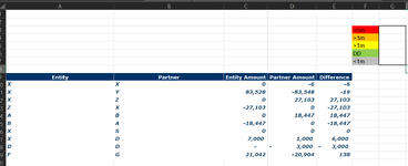
I'm trying to populate the cells in the column G (>5m, >3m etc), based on the difference column which is in Millions and also highlight column E based on the below.

I want any differences that nets two 0 (e.g XZ and ZX) and any difference <1m to be highlighted in Grey and the sum of these to put next to the "<1m" in the column G.
Any difference that are >1m but less <3m and <-1m but >-3m to be highlighted in Yellow and the sum of these put next to the ">1m" in the column G.
Any difference that are >3m but less <5m and <-3m but >-5m to be highlighted in Orange and the sum of these put next to the ">3m" in the column G.
Any difference that are >5m and <-5m to be highlighted in Red and the sum of these put next to the ">5m" in the column G.
Any difference where the entity and partner are both "D" to be highlighted in Green and the sum of these put next to the "DD".

Column G should be filled on an absolute basis, for example in cell G7 the final result would be the sum of E10, E11 and E19.

I want this automated to the point where I just copy and paste the data which will vary each time in terms of the number of rows (number of columns will stay the same) into columns A to E and column G fills automatically and column E is also colour coded as above.

I've been trying to figure it out but can only do certain bits and can't get the whole picture. I'm not sure if this is possible or not.
 

Attachments

  • Example 2.png
    Example 2.png
    34.1 KB · Views: 13

Excel Facts

VLOOKUP to Left?
Use =VLOOKUP(A2,CHOOSE({1,2},$Z$1:$Z$99,$Y$1:$Y$99),2,False) to lookup Y values to left of Z values.
Is the data in columns C, D and E in millions?

The first part, the formatting of with conditional formatting to highlight the colours.
As a simple step, you can use some helper columns to then include the values based on the same formulas for the conditional formatting, sum the columns and have the relevent cells in column G = the sum of that helper column
I want any differences that nets two 0 (e.g XZ and ZX) and any difference <1m to be highlighted in Grey and the sum of these to put next to the "<1m" in the column G.
Any difference that are >1m but less <3m and <-1m but >-3m to be highlighted in Yellow and the sum of these put next to the ">1m" in the column G.
Any difference that are >3m but less <5m and <-3m but >-5m to be highlighted in Orange and the sum of these put next to the ">3m" in the column G.
Any difference that are >5m and <-5m to be highlighted in Red and the sum of these put next to the ">5m" in the column G.
Any difference where the entity and partner are both "D" to be highlighted in Green and the sum of these put next to the "DD".

I don't follow how the values for 1m, 3m, etc are calculated based on the data provided. None of the figures in cols D, E, F are in the millions.
You can use a SUM and an IF function rather than a helper column also, eg, in G5 put:
=SUMIFS(E10:E19,E10:E19,">-3000000",E10:E19,"<-1000000") + SUMIFS(E10:E19,E10:E19,">1000000",E10:E19,"3000000")

Also, when you say "Column G should be filled on an absolute basis, for example in cell G7 the final result would be the sum of E10, E11 and E19", what do you mean by absolute. The ABS function will return the absolute value
EG,
=ABS(SUM(C11:E11)) would return the absolute value of the sum of those three cells, being +39, whereas =(SUM(C11:E11) would return the SUM of the 3 cells as -39.
Summing the absolute values of those three cells though, like so =ABS(C11)+ABS(D11)+ABS(E11) gives the answer of 167095
Hence why it is important to understand which one you mean when you say the "absolute basis"

Cheers
 
Upvote 0
Is the data in columns C, D and E in millions?

The first part, the formatting of with conditional formatting to highlight the colours.
As a simple step, you can use some helper columns to then include the values based on the same formulas for the conditional formatting, sum the columns and have the relevent cells in column G = the sum of that helper column


I don't follow how the values for 1m, 3m, etc are calculated based on the data provided. None of the figures in cols D, E, F are in the millions.
You can use a SUM and an IF function rather than a helper column also, eg, in G5 put:
=SUMIFS(E10:E19,E10:E19,">-3000000",E10:E19,"<-1000000") + SUMIFS(E10:E19,E10:E19,">1000000",E10:E19,"3000000")

Also, when you say "Column G should be filled on an absolute basis, for example in cell G7 the final result would be the sum of E10, E11 and E19", what do you mean by absolute. The ABS function will return the absolute value
EG,
=ABS(SUM(C11:E11)) would return the absolute value of the sum of those three cells, being +39, whereas =(SUM(C11:E11) would return the SUM of the 3 cells as -39.
Summing the absolute values of those three cells though, like so =ABS(C11)+ABS(D11)+ABS(E11) gives the answer of 167095
Hence why it is important to understand which one you mean when you say the "absolute basis"

Cheers
Sorry, wrote the post late last night.

Columns C,D,E have been divided by 1000. So E10 is -6000 for example.

Ignore the absolute basis comment, that is wrong on my part.
 
Upvote 0

Forum statistics

Threads
1,215,131
Messages
6,123,222
Members
449,091
Latest member
jeremy_bp001

We've detected that you are using an adblocker.

We have a great community of people providing Excel help here, but the hosting costs are enormous. You can help keep this site running by allowing ads on MrExcel.com.
Allow Ads at MrExcel

Which adblocker are you using?

Disable AdBlock

Follow these easy steps to disable AdBlock

1)Click on the icon in the browser’s toolbar.
2)Click on the icon in the browser’s toolbar.
2)Click on the "Pause on this site" option.
Go back

Disable AdBlock Plus

Follow these easy steps to disable AdBlock Plus

1)Click on the icon in the browser’s toolbar.
2)Click on the toggle to disable it for "mrexcel.com".
Go back

Disable uBlock Origin

Follow these easy steps to disable uBlock Origin

1)Click on the icon in the browser’s toolbar.
2)Click on the "Power" button.
3)Click on the "Refresh" button.
Go back

Disable uBlock

Follow these easy steps to disable uBlock

1)Click on the icon in the browser’s toolbar.
2)Click on the "Power" button.
3)Click on the "Refresh" button.
Go back
Back
Top