Using XLookup on two lists with VStack and Filter

[Zakky]

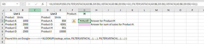
Hello. I have been looking into using Xlookup for data on two different lists. I managed to find a solution on Google but can't get it to work following several failed attempts. I am trying to get the sales for a product in cell G1. A bonus would be, as a separate exercise, if i can use SUMIFS to get a sum of sales for product A (appears on both lists). Many thanks!

 

[awoohaw]

try using FILTER instead of XLOOKUP, for all your scenarios.

Book1
	A	B	C	D	E	F	G	H
1						Product	G
2	Product	Units		Product	Units		6581	Using cell G1
3	ProductA	1050		ProductA	850		6581	Prod G
4	ProductB	2000		ProductG	6581		1900	Prod A
5	ProductC	500		ProductH	951
6	ProductD	2500		ProductI	15000
Sheet5

Cell Formulas
Range	Formula
G2	G2	=SUM(LET(arr,VSTACK($A$3:$B$6,$D$3:$E$6),trgt,"Product"&$G$1,prd,TAKE(arr,,1),amts,TAKE(arr,,-1),FILTER(amts,prd=trgt,"")))
G3	G3	=SUM(LET(arr,VSTACK($A$3:$B$6,$D$3:$E$6),trgt,"Product"&"G",prd,TAKE(arr,,1),amts,TAKE(arr,,-1),FILTER(amts,prd=trgt,"")))
G4	G4	=SUM(LET(arr,VSTACK($A$3:$B$6,$D$3:$E$6),trgt,"Product"&"A",prd,TAKE(arr,,1),amts,TAKE(arr,,-1),FILTER(amts,prd=trgt,"")))

 

[KRice]

another option...

MrExcel_20240224.xlsx
	A	B	C	D	E	F	G	H
1	List 1			List 2
2	Product	Units		Product	Units		951	H
3	A	1050		A	850		1900	A
4	B	2000		G	6581
5	C	500		H	951
6	D	2500		I	1500
Sheet7

Cell Formulas
Range	Formula
G2:G3	G2	=LET(comb,VSTACK($A$3:$B$6,$D$3:$E$6),SUM(FILTER(TAKE(comb,,-1),TAKE(comb,,1)=$H2)))

Edit:...essentially the same as @awoohaw's in a slightly different order

 

[awoohaw]

another option...

MrExcel_20240224.xlsx
	A	B	C	D	E	F	G	H
1	List 1			List 2
2	Product	Units		Product	Units		951	H
3	A	1050		A	850		1900	A
4	B	2000		G	6581
5	C	500		H	951
6	D	2500		I	1500
Sheet7

Cell Formulas
Range	Formula
G2:G3	G2	=LET(comb,VSTACK($A$3:$B$6,$D$3:$E$6),SUM(FILTER(TAKE(comb,,-1),TAKE(comb,,1)=$H2)))

Edit:...essentially the same as @awoohaw's in a slightly different order

and more concise, i realized I could have made it smaller after I posted.

 

[Zakky]

KRice & awoohaw, Thank you for your prompt replies. The solutions are a bit different from what i was expecting, but they both work for me, so win is a win. Once again, many thanks!

 

[awoohaw]

KRice & awoohaw, Thank you for your prompt replies. The solutions are a bit different from what i was expecting, but they both work for me, so win is a win. Once again, many thanks!

well, xlookup will not find a second value so that was not going to be in a solution. You're welcome. Best wishes.

 

[KRice]

Glad we could help!