VBA Code Help

[tinneytwin]

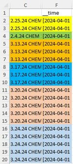
I need a VBA Code that will first look at the rows in Column F for matching data AND look in Column C for matching data (F & C will never match). For instance, if F2, F3, F4, F5, and F6 all match, then it needs to look in C2, C3, C4, C5, C6. For the rows in C that match (with the corresponding F matches), I need them to be highlighted. And keep repeating that pattern until all rows are highlighted.

I have a small portion of the data pictured here to show what I mean because it's hard to explain. In my picture, all column F are the same (only because this is a small portion of the data) but column C is different so I have them grouped/highlighted by F first then C. Column C is the name of a video and Column F is a date (with other information that I have truncated). The excel document will have thousands of rows it will need to go through and highlight. Right now I do this manually and it takes me forever because I have 26 different excel documents with thousands of rows in each document. I originally got VBA macro codes from someone who said they knew how to code macros, but none of their macro coding worked. I know nothing about coding.
(the colors don't have to be different. It could rotate back and forth between two colors)

 

[myall_blues]

If you don't mind using another column you could do this with conditional formatting and dispense with the VBA code. The first row of interest in column H is simply set to true, and then the subsequent rows in column H contain a formula

=IF(AND(F3=F2,C3=C2),H2,NOT(H2))

The conditional formatting is then just based on whether the value in H is TRUE or FALSE.

tinneytwin.xlsx
	B	C			F	G	H
1
2		2.25.24 CHEM			[2024-04-01]		TRUE
3		2.25.24 CHEM			[2024-04-01]		TRUE
4		2.4.24 CHEM			[2024-04-01]		FALSE
5		3.13.24 CHEM			[2024-04-01]		TRUE
6		3.13.24 CHEM			[2024-04-01]		TRUE
7		3.13.24 CHEM			[2024-04-01]		TRUE
8		3.17.24 CHEM			[2024-04-01]		FALSE
9		3.17.24 CHEM			[2024-04-01]		FALSE
10		3.17.24 CHEM			[2024-04-01]		FALSE
11		3.20.24 CHEM			[2024-04-01]		TRUE
12		3.20.24 CHEM			[2024-04-01]		TRUE
13		3.20.24 CHEM			[2024-04-01]		TRUE
14		3.20.24 CHEM			[2024-04-02]		FALSE
15		3.20.24 CHEM			[2024-04-03]		TRUE
Sheet1

Cell Formulas
Range	Formula
H2	H2	=TRUE()
H3:H15	H3	=IF(AND(F3=F2,C3=C2),H2,NOT(H2))

Cells with Conditional Formatting
Cell	Condition		Cell Format	Stop If True
C2:F15	Expression	=$H2=FALSE	text	NO
C2:F15	Expression	=$H2	text	NO

Credit to the late Chip Pearson where I originally learned this idea.

 

[tinneytwin]

If you don't mind using another column you could do this with conditional formatting and dispense with the VBA code. The first row of interest in column H is simply set to true, and then the subsequent rows in column H contain a formula

=IF(AND(F3=F2,C3=C2),H2,NOT(H2))

The conditional formatting is then just based on whether the value in H is TRUE or FALSE.

tinneytwin.xlsx
	B	C			F	G	H
1
2		2.25.24 CHEM			[2024-04-01]		TRUE
3		2.25.24 CHEM			[2024-04-01]		TRUE
4		2.4.24 CHEM			[2024-04-01]		FALSE
5		3.13.24 CHEM			[2024-04-01]		TRUE
6		3.13.24 CHEM			[2024-04-01]		TRUE
7		3.13.24 CHEM			[2024-04-01]		TRUE
8		3.17.24 CHEM			[2024-04-01]		FALSE
9		3.17.24 CHEM			[2024-04-01]		FALSE
10		3.17.24 CHEM			[2024-04-01]		FALSE
11		3.20.24 CHEM			[2024-04-01]		TRUE
12		3.20.24 CHEM			[2024-04-01]		TRUE
13		3.20.24 CHEM			[2024-04-01]		TRUE
14		3.20.24 CHEM			[2024-04-02]		FALSE
15		3.20.24 CHEM			[2024-04-03]		TRUE
Sheet1

Cell Formulas
Range	Formula
H2	H2	=TRUE()
H3:H15	H3	=IF(AND(F3=F2,C3=C2),H2,NOT(H2))

Cells with Conditional Formatting
Cell	Condition		Cell Format	Stop If True
C2:F15	Expression	=$H2=FALSE	text	NO
C2:F15	Expression	=$H2	text	NO

Credit to the late Chip Pearson where I originally learned this idea.

THANK YOU SO MUCH!!! You saved me so much time!

 

[myall_blues]

You’re welcome. Thanks for the feedback.