VBA to return "1" if a word in a cell is red

ferrigeu

Board Regular
Joined
Jun 14, 2017
Messages
50
Office Version
  1. 2016
Platform
  1. Windows
hi all
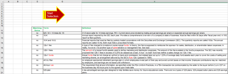
i have a good VBA looking for a word (or multiple words separated by comma, via an entry box) that looks in two columns (columns G and H, in an xls file and highlights said word(s) in red (changes the font from black to red). ONLY the word that i am searching for is highlighted, not the entire content of the cell (e.g. g17, h24, g25, h25, etc. is where the word(s) are found).
this has worked well in the past.... but the requirements have now changed....
new: i need to have a "1" in column B for each/all cells where a word(s) in that cell is highlighted in red (e.g. b17, b24) and for rows where there are red words in G25 and h25, it needs to be a 2. i don't need to count the number of instances a word is red (so if "the" is highlighted red 4 times in g25 and 7 times in h25, i need to see 2, not 11)
any thoughts pls?
doable?
apologies - we have a super tight IT and not export, send, etc. from the work environment
i have tried to add screenshots, but they are too large to post

thank you
 

Excel Facts

Formula for Yesterday
Name Manager, New Name. Yesterday =TODAY()-1. OK. Then, use =YESTERDAY in any cell. Tomorrow could be =TODAY()+1.
Hello @ferrigeu.

I want to make some notes:
  1. i need to have a "1" in column B for each/all cells where a word(s) in that cell is highlighted in red (e.g. b17, b24)
    I guess those cells must be G17 and H24, correct?


  2. i have a good VBA looking for a word (or multiple words separated by comma, via an entry box)
    It would be great if you put that macro here, that way it would be enough to make the change and you would have the 2 processes in a single macro. 🤷‍♂️


  3. i have tried to add screenshots, but they are too large to post
    It is not necessary to put the whole screen, only with a sample of columns B, G and H, the other columns can be hidden. 😎
    Example:
    1681869344452.png


Since we don't have the original macro, then you will have a separate macro.
Then try the following macro. The macro checks each cell in columns G and H and checks if any words are in red.
VBA Code:
Sub Return_1_2()
  Dim c As Range
  Dim i As Long, b1 As Long, b2 As Long
 
  For Each c In Range("G2", Range("G" & Rows.Count).End(3))
    b1 = 0
    b2 = 0
    For i = 1 To Len(c.Value)
      If c.Characters(i, 1).Font.Color = vbRed Then
        b1 = 1
        Exit For
      End If
    Next
    For i = 1 To Len(c.Offset(, 1).Value)
      If c.Offset(, 1).Characters(i, 1).Font.Color = vbRed Then
        b2 = 1
        Exit For
      End If
    Next
    Range("B" & c.Row).Value = b1 + b2
  Next
End Sub

--------------
Let me know the result and I'll get back to you as soon as I can.
Sincerely
Dante Amor
--------------
 
Upvote 0
Solution
Hello @ferrigeu.

I want to make some notes:

  1. I guess those cells must be G17 and H24, correct?


  2. It would be great if you put that macro here, that way it would be enough to make the change and you would have the 2 processes in a single macro. 🤷‍♂️


  3. It is not necessary to put the whole screen, only with a sample of columns B, G and H, the other columns can be hidden. 😎
    Example:
    View attachment 89995


Since we don't have the original macro, then you will have a separate macro.
Then try the following macro. The macro checks each cell in columns G and H and checks if any words are in red.
VBA Code:
Sub Return_1_2()
  Dim c As Range
  Dim i As Long, b1 As Long, b2 As Long
 
  For Each c In Range("G2", Range("G" & Rows.Count).End(3))
    b1 = 0
    b2 = 0
    For i = 1 To Len(c.Value)
      If c.Characters(i, 1).Font.Color = vbRed Then
        b1 = 1
        Exit For
      End If
    Next
    For i = 1 To Len(c.Offset(, 1).Value)
      If c.Offset(, 1).Characters(i, 1).Font.Color = vbRed Then
        b2 = 1
        Exit For
      End If
    Next
    Range("B" & c.Row).Value = b1 + b2
  Next
End Sub

--------------
Let me know the result and I'll get back to you as soon as I can.
Sincerely
Dante Amor
--------------
hi Dante
i included your suggestion
works good - but it hung excel every time i ran it (maybe because the table has about 22150 lines?)
below is the code i have at this time, and a screenshot...
alternatively, and now that i think about it, instead of adding and running this code, would it be possible to 'store' each search criteria in a new cell (a1, a2, a3, etc) and then i can add a formula with SEARCH - that will go through it quicker i think....?


Sub HighlightStrings()
'Updateby Extendoffice

'sort the data
Call sorting

'change font back to black
ActiveSheet.Range("g12:h22500").Select
Range("g12:h22500").Font.ColorIndex = 1

'set parameters
Dim Rng As Range
Dim cFnd As String
Dim xTmp As String
Dim x As Long
Dim m As Long
Dim y As Long
Dim xFNum As Integer
Dim xArrFnd As Variant
Dim xStr As String
cFnd = InputBox("Please enter the text, separate them by comma:")
If Len(cFnd) < 1 Then Exit Sub

'not case sensitive
xArrFnd = Split(UCase(cFnd), ",")

'case sensitive
'xArrFnd = Split(cFnd, ",")

'define the range of the data
ActiveSheet.Range("g12:h22500").Select

For Each Rng In selection
With Rng
For xFNum = 0 To UBound(xArrFnd)
xStr = xArrFnd(xFNum)
y = Len(xStr)
m = UBound(Split(UCase(Rng.Value), UCase(xStr)))

'case sensitive
'm = UBound(Split(Rng.Value, xStr))


If m > 0 Then
xTmp = ""
For x = 0 To m - 1

xTmp = xTmp & Split(UCase(Rng.Value), UCase(xStr))(x)

'case sensitive
'xTmp = xTmp & Split(UCase(Rng.Value), UCase(xStr))(x)

.Characters(Start:=Len(xTmp) + 1, Length:=y).Font.ColorIndex = 3
xTmp = xTmp & xStr
Next
End If
Next xFNum
End With
Next Rng

Application.ScreenUpdating = True

'cursor goes back
Range("h7").Select

End Sub
Sub sorting()
'
' sorting Macro
'
'
Range("g12:h22500").Select
ActiveWorkbook.Worksheets("Almanac").Sort.SortFields.Clear
ActiveWorkbook.Worksheets("Almanac").Sort.SortFields.Add Key:=Range( _
"G12:G22500"), SortOn:=xlSortOnValues, Order:=xlAscending, DataOption:= _
xlSortNormal
ActiveWorkbook.Worksheets("Almanac").Sort.SortFields.Add Key:=Range( _
"H12:H22500"), SortOn:=xlSortOnValues, Order:=xlAscending, DataOption:= _
xlSortNormal
With ActiveWorkbook.Worksheets("Almanac").Sort
.SetRange Range("G11:H3524")
.Header = xlYes
.MatchCase = False
.Orientation = xlTopToBottom
.SortMethod = xlPinYin
.Apply
End With
End Sub


screenshot:
1681907708759.png
 

Attachments

  • 1681906815878.png
    1681906815878.png
    53.3 KB · Views: 3
Upvote 0
Hi @ferrigeu.

What you are asking for are new requirements that are not in your original post.

I suggest the following:
1. Create a new post.
2. In the new post explain what changes you need.
3. Put the macro in the new post:
Note Code Tag:
In future please use code tags when posting code.​
How to Post Your VBA Code it makes your code easier to read and copy and it also maintains VBA formatting.​

4. Put an image or a minisheet using the XL2BB tool of the cells with the criteria:
Note XL2BB:
For the future, it would help greatly if you could give us the sample data in a form that we can copy to test with, rather that a picture.​
MrExcel has a tool called “XL2BB” that lets you post samples of your data that will allow us to copy/paste it to our Excel spreadsheets, so we can work with the same copy of data that you are. Instructions on using this tool can be found here: XL2BB Add-in
Note that there is also a "Test Here” forum on this board. This is a place where you can test using this tool (or any other posting techniques that you want to test) before trying to use those tools in your actual posts.​

5. Put an image of how your data is before the macro
6. Put another image of the desired result.
If I have time, it will be my pleasure to help you.
 
Upvote 0

Forum statistics

Threads
1,214,979
Messages
6,122,560
Members
449,089
Latest member
Motoracer88

We've detected that you are using an adblocker.

We have a great community of people providing Excel help here, but the hosting costs are enormous. You can help keep this site running by allowing ads on MrExcel.com.
Allow Ads at MrExcel

Which adblocker are you using?

Disable AdBlock

Follow these easy steps to disable AdBlock

1)Click on the icon in the browser’s toolbar.
2)Click on the icon in the browser’s toolbar.
2)Click on the "Pause on this site" option.
Go back

Disable AdBlock Plus

Follow these easy steps to disable AdBlock Plus

1)Click on the icon in the browser’s toolbar.
2)Click on the toggle to disable it for "mrexcel.com".
Go back

Disable uBlock Origin

Follow these easy steps to disable uBlock Origin

1)Click on the icon in the browser’s toolbar.
2)Click on the "Power" button.
3)Click on the "Refresh" button.
Go back

Disable uBlock

Follow these easy steps to disable uBlock

1)Click on the icon in the browser’s toolbar.
2)Click on the "Power" button.
3)Click on the "Refresh" button.
Go back
Back
Top