XLOOKUP - Lookup Value is a formula

[p33lcg]

Hello,

I am having some problems using XLOOKUP as my lookup value is generated by a formula, I am therefore getting the dreaded #NA. The formula works and the value is definitely in the array as if I manually type the value, it can find it.

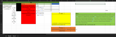
I am trying to use the value in F3 which has the below formula in:

=IF(ISBLANK(B3),"",MID(B3,FIND("Member:",B3)+7,FIND("Automated",B3)-FIND("Member:",B3)-7))

The XLOOKUP Formula is:

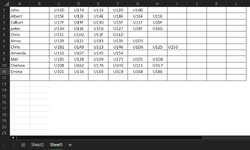
=IFERROR(IFERROR(IFERROR(IFERROR(IFERROR(IFERROR(IFERROR(IFERROR(XLOOKUP(F3, Sheet1!C:C, Sheet1!A:A), XLOOKUP(F3, Sheet1!D:D, Sheet1!A:A)), XLOOKUP(F3, Sheet1!E:E, Sheet1!A:A)), XLOOKUP(F3, Sheet1!F:F, Sheet1!A:A)), XLOOKUP(F3, Sheet1!G:G, Sheet1!A:A)), XLOOKUP(F3, Sheet1!H:H, Sheet1!A:A)), XLOOKUP(F3, Sheet1!I:I, Sheet1!A:A)), XLOOKUP(F3, Sheet1!J:J, Sheet1!A:A)), XLOOKUP(F3, Sheet1!K:K, Sheet1!A:A))

As a note, F3 produces a code such as "R4G6" and the lookup produces a name.

Any help would be much appreciated.

P.s any tips on getting the long formulas shortened would also be welcomed if possible!

 

[Dave Patton]

Review the formula information for XLookup.

try

XLookup.xlsm
	F	G
1
2
3	R4G6	ABCD
4
6e

Cell Formulas
Range	Formula
G3	G3	=XLOOKUP(F3, Sheet1!C:C, Sheet1!A:A,"",0)

You could make a small example and then try Formulas Formula Evaluate

N.B. You can post a concise example of your sheet with the forum's tool named XL2BB.

You may not need full column references; consider a reasonable number considering your data.

 

[Dave Patton]

1. We do not know your data.
2. We do not know what you are trying to do.

3. There are variety of different approaches explained on the internet.

5. One idea is to consolidate your data ranges with Vstack and then use XLookup or another formula
My example uses multiple sheets but the idea works with multiple ranges or tables.

XLookup.xlsm
	F	G	H	I	J	K	L	M
3	R4G6		ABCD			0	0	0
6e

Cell Formulas
Range	Formula
H3	H3	=XLOOKUP(F3, M3:M44,K3:K44,"",0)
K3:M44	K3	=VSTACK(Sheet1!A2:C20,Sheet2!A2:C24)
Dynamic array formulas.

 

[Fluff]

Hi & welcome to MrExcel.
How about

=TAKE(TOCOL(IF(Sheet1!C$2:K$1000=F3,Sheet1!A$2:A$1000,1/0),2),1)

 

[p33lcg]

Hello Both,

Thanks for your responses, unfortunately neither have worked.

I can't use XL2BB as states doesn't work on protected workbooks (work PC), I have though put the examples in a screenshot to give some clarity, the formulas for each are underneath.

On the actual sheet I'm using, there is around 100 rows, but won't have duplicates

Thank you again.

 

[Fluff]

With the TOCOL/IF approach you should have the ranges the same number of rows.
That said it would not give an error unless the value in E3 was not found. Check that it does not have any leading/trailing spaces or other hidden characters.

 

[p33lcg]

Hi Fluff,

You're a star thank you! Have sorted it, you're right is because there was a hidden space in E3 value, I have adjusted the E3 formula and works sweet now.

Thank you

 

[Fluff]

Glad we could help & thanks for the feedback.