Dynamic Top/bottom calculation

[alizok]

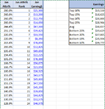
I need the assistance of this group in developing a formula that will dynamically modify dependent on the number of records in the database. I need to figure out the top 10%, top 25%, top 30%, bottom 10%, bottom 25%, and so on. Is there a formula that can automatically calculate this information? Typically, I rank the data, then sort it from smallest to largest, and then determine the average of a certain data set manually depending on the percentage. see attached for more details.

Thank you in advance for all your help

 

[alizok]

Thanks for that.
How about

Fluff.xlsm
	A	B	C	D
1
2
3			count	Results
4	Top 10		5	£26,800
5	Top 25%		13	£36,690
6	Avg			£30,054
7	Bottom 25%		13	£20,667
8	Bottom 10%		5	£14,200
9
10		Total count	53
11		Jan Attn%	Jan Attn% Rank	Jan Earning
12		97.20%	42	15,475
13		244.40%	5	67,500
14		191.50%	13	78,300
15		166.70%	14	56,875
16		215.60%	9	78,850
17		151.10%	19	47,550
18		195.60%	11	69,850
19		115.60%	30	43,225
20		137.80%	22	44,425
21		148.90%	20	45,200
22		88.90%	44	14,950
23		153.30%	17	43,175
24		84.40%	47	17,025
25		130.50%	23	32,575
26		86.70%	45	27,775
27		104.40%	33	22,925
28		117.80%	29	24,175
29		97.80%	41	43,300
30		84.40%	47	12,150
31		102.20%	34	27,350
32		128.90%	24	46,975
33		84.40%	47	23,325
34		111.10%	32	25,425
35		102.20%	34	39,375
36		113.60%	31	30,275
37		194.40%	12	22,225
38		83.30%	51	11,750
39		81.00%	52	2,650
40		91.50%	43	54,525
41		166.70%	14	23,650
42		151.80%	18	49,800
43		118.60%	28	35,225
44		84.40%	47	16,275
45		100.00%	36	5,050
46		86.70%	45	12,475
47		280.00%	1	25,900
48		100.00%	36	29,650
49		260.00%	2	13,200
50		200.00%	10	12,425
51		220.00%	7	33,550
52		100.00%	36	20,500
53		100.00%	36	17,100
54		260.00%	2	14,650
55		260.00%	2	12,750
56		220.00%	7	8,350
57		160.00%	16	26,325
58		120.00%	25	26,075
59		80.00%	53	17,000
60		140.00%	21	19,850
61		100.00%	36	27,925
62		120.00%	25	10,950
63		231.10%	6	39,425
64		120.00%	25	25,575
Main

Cell Formulas
Range	Formula
D4:D8	D4	=LET(data,SORT(C12:D64),r,ROWS(data),VSTACK(AVERAGE(TAKE(data,r*0.1,-1)),AVERAGE(TAKE(data,r*0.25,-1)),AVERAGE(TAKE(data,,-1)),AVERAGE(TAKE(data,-r*0.25,-1)),AVERAGE(TAKE(data,-r*0.1,-1))))
Dynamic array formulas.

I'm trying to understand this formula. would you please explain it a bit.

 

[alizok]

I figured out the formula. Thank you and it's working like a charm. Is there a way to adjust this formula to account for the ties?

 

[Fluff]

Not sure what you mean by accounting for ties, but it would be better to start a new thread for this question.