Excel Blood Pressure & Heart Rate AVG?

[puw]

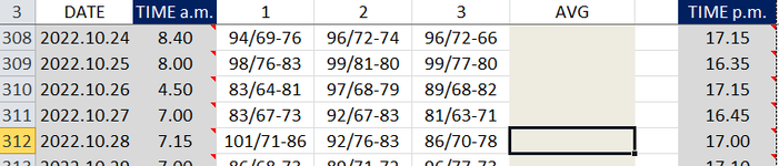
Twice a day I take my BP & heart rate. Each time I take 3 tests and then manually AVG.

The format I use in each column for the digital testing machine's results is S/D-H (85/70-81).

Because this is a standard way of showing these 3 measurements and because with a total of 6 measurements a day ... plus additional data, I want to keep to this format so that I can easily input and see ALL data I input on a screen without left/right scrolling (not spread out over multiple columns for individual numbers taking up too much width with all the additional data - which I know now would make it so much easier to do, but I do not have time now to reset all the data).

I came across this thread BP Excel Formula and have tried to change what I think should be changed but since I have a 'LEFT', a 'MIDDLE' and a 'RIGHT' number along with the '/' & '-' x 3 for each test, I cannot work out how to alter it to work. Unfortunately I am not very good when it comes to working out a formula for such data.

The data collected up to now covers almost 12 months - so there is a lot.

Occasionally I am too busy and 'miss' a test.

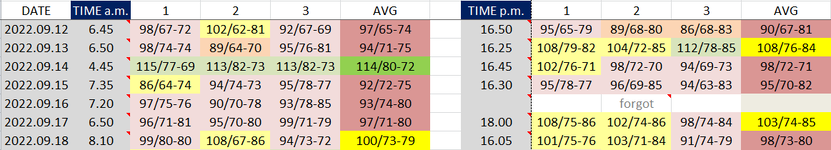
I have a colour code range that reflects the SYSTOLIC result only (that's the high number of the two ref. BP) ... but I am not sure this is available via using a formula because each result is a lighter shade of a main colour, the main colour being the one used for the average.

Can anyone please help me know if Excel can handle a formula for the way I input the data to create an AVG automatically. Can anyone help me to create the formula please? If it is possible, then I would like to link the AVG results to a 2nd sheet to show a chart. Due to where I live and COVID, it has not been possible for me to get back to see the doctor since the beginning of the year and I collect this data so as when I can get to see them, they will have an easy identifiable way of seeing how my health has been doing over this last year via the medication they initially set me on and whether they prefer the numbers or a chart, they can hopefully deduce future treatment more easily from my daily records. For my benefit, it would make my task of record keeping much easier & time efficient (because it takes quite a bit of time to input ALL of the data I collect and record, AVG the results, colour code as per images below etc).

Many thanks and I've included some screen shots that I hope will help you understand.

 

[Leo Skywalker]

Hi there,

This formula will get the average you want in one cell, however, in order to extract any useful information for a chart, you would have to resort to individual calculations as the ones already provided, maybe in some far right columns, hidden from view.

E3:

=ROUND(AVERAGE(VALUE(LEFT(B3:D3,FIND("/",B3:D3)-1))),0)&"/"&ROUND(AVERAGE(VALUE(MID(B3:D3,FIND("/",B3:D3)+1,FIND("-",B3:D3)-FIND("/",B3:D3)-1))),0)&"-"&ROUND(AVERAGE(VALUE(RIGHT(B3:D3,LEN(B3:D3)-FIND("-",B3:D3)))),0)

This is an array formula, so if the Excel version is not 365, will need to have CTRL+SHIFT+ENTER.

 

[puw]

Hi there,

This formula will get the average you want in one cell, however, in order to extract any useful information for a chart, you would have to resort to individual calculations as the ones already provided, maybe in some far right columns, hidden from view.


View attachment 77715
E3:

=ROUND(AVERAGE(VALUE(LEFT(B3:D3,FIND("/",B3:D3)-1))),0)&"/"&ROUND(AVERAGE(VALUE(MID(B3:D3,FIND("/",B3:D3)+1,FIND("-",B3:D3)-FIND("/",B3:D3)-1))),0)&"-"&ROUND(AVERAGE(VALUE(RIGHT(B3:D3,LEN(B3:D3)-FIND("-",B3:D3)))),0)

This is an array formula, so if the Excel version is not 365, will need to have CTRL+SHIFT+ENTER.

Thank you for the above information - your explanation of what a chart needs leads me more and more in David's direction of simplifying the data ... start over but extract some 300 entries to individual cells for each test result number (24 columns vs 8). Thank you

 

[puw]

You have provided good information. It is a challenge providing suggestions when I do not know the data, background, goals, constraints, etc.

You stated "an easy way to extract the original data format of 95/82-89 to individual cells". I believe my suggestions may help with this.
Some of the formula get more complex if there is a mix of 2 and 3 character numbers.
Some of the formulas may require array enter unless you have Excel 365 or 2021.

"see how and if the shading/colouring of cells gives the same/right instant visual appearance."
Excel can colour cells via conditional formatting. For example if cell is >150 highlight in Red.

N.B. Please consider downloading the forum's tool called XL2BB. You will then be able to provide an extract of your sheet.

I updated some of the suggestions. I used an older version of Excel; the array formulas will now be highlighted.

The suggestions and formatting are not organized. Pull the information that seems useful. Ask questions.

You can copy my Excel extract to a clean sheet. Click on the icon below the f(x) in the heading and then move to your sheet and paste.

Dear David,
I'm glad the additional details were helpful to you. Thank you so much David.

Some may very well 'throw the towel in' at this point, but to be honest with so much data now accrued, it needs a simpler form of presentation I feel via a chart, that since we see everything in pictures first will benefit all intended participants. I know I was hoping the mountain might come to me, but I see now it has to be the reverse via a clean sheet, extract, apply formulas, create charts.

I will hang on on uploading my table as I'm the kind of person who wants to work out (with your help) how to do it first. Besides, I would have to remove a lot of personal info first which I do not want to share publicly. I am familiar with and have used for many years (personal) ASAP Utilities, which I think will be of great help to me yet again in doing this, as it has so many times over the years.

I'm sure this is going to take a good few days for me to work through, fail, questions, try another of your alternatives for a solution, perhaps find a solution through a combination etc ... so please forgive my absence - I will not be ignoring you or the other members helping me ... I just need to clear my head, focus on the job ahead, get the data extracted into a visual format I can live with and then apply the AVG formulas that make it simple and that will give the right chart etc.

Thank you

 

[Dave Patton]

Revision 2
A.
Log of Blood Pressure moving forward
Columns L:N provide the average of the 3 readings * 2
First post shows the result with hidden columns. Does this work on your systems?
Do you want just one number a day (average of the 2 sets of readings)?
The second part shows the detail and an alternative for the data entry.
Which order of entry do you prefer?
B.
Extract of information from the data already recorded.
If there are always 3 numbers, this version does not require Array Enter.

I can post Revision 1 if you want me to.

T202211a.xlsm
	A											L	M	N
1	Future Daily Log											Average
2	Date											D	S	P
3	2-Nov-22											102	71	72
4	2-Nov-22											104	71	73
5	3-Nov-22											96	71	59
6	3-Nov-22											105	74	61
7	4-Nov-22											118	72	63
8	4-Nov-22											103	72	61
9	or
10	Date
11	2-Nov-22											102	71	72
12
2aa

Cell Formulas
Range	Formula
L3:L8	L3	=AVERAGE(C3:E3)
M3:M8	M3	=AVERAGE(F3:H3)
N3:N8	N3	=AVERAGE(I3:K3)
L11:N11	L11	=AVERAGE(C11,F11,I11)

detail I can delete column B; it does not yield values that we can use.

T202211a.xlsm
	A	B	C	D	E	F	G	H	I	J	K	L	M	N
1	Future Daily Log											Average
2	Date	Result	D-1	D-2	D-3	S-1	S-2	S-3	P-1	P-2	P-3	D	S	P
3	2-Nov-22	102/71-72	115	96	96	69	72	72	76	74	66	102	71	72
4	2-Nov-22	104/71-73	120	96	96	69	72	72	76	74	70	104	71	73
5	3-Nov-22	96/71-59	99	95	94	71	71	71	60	59	58	96	71	59
6	3-Nov-22	105/74-61	125	95	94	71	80	71	60	65	58	105	74	61
7	4-Nov-22	118/72-63	125	120	110	70	77	70	62	63	64	118	72	63
8	4-Nov-22	103/72-61	80	120	110	70	77	70	55	63	64	103	72	61
9	or
10	Date	Result	D-1	S-1	P-1	D-2	S-2	P-2	D-3	S-3	P-3
11	2-Nov-22	102/71-72	115	69	76	96	72	74	96	72	66	102	71	72
12
2aa

Cell Formulas
Range	Formula
L3:L8	L3	=AVERAGE(C3:E3)
M3:M8	M3	=AVERAGE(F3:H3)
N3:N8	N3	=AVERAGE(I3:K3)
B3:B8	B3	=ROUND(AVERAGE(C3:E3),0)&"/"&ROUND(AVERAGE(F3:H3),0)&"-"&ROUND(AVERAGE(I3:K3),0)
B11	B11	=ROUND(AVERAGE(C11,F11,I11),0)&"/"&ROUND(AVERAGE(D11,G11,J11),0)&"-"&ROUND(AVERAGE(E11,H11,K11),0)
L11:N11	L11	=AVERAGE(C11,F11,I11)

Extract from previously recorded information

T202211a.xlsm
	A	B	C	D	E	F	G
13	Revison 2
14	Date	#1	#2	#3	Diastolic	Systolic	Pulse
15	31-Aug-22	94/69-76	96/72-74	96/72-66	95	71	72
16	1-Sep-22	98/69-76	96/72-74	99/72-66	98	71	72
17	2-Sep-22	115/69-72	96/72-74	99/70-68	103	70	71
18	3-Sep-22	120/70-66	96/72-74	99/70-104	105	71	81
19
2a

Cell Formulas
Range	Formula
E15:E18	E15	=SUMPRODUCT(--MID(B15:D15,1,FIND("/",B15:D15)-1))/3
F15:F18	F15	=SUMPRODUCT(--MID(B15:D15,FIND("/",B15:D15)+1,2))/3
G15:G18	G15	=SUMPRODUCT(--MID(B15:D15,FIND("-",B15:D15)+1,99))/3

 

[Dave Patton]

Good morning
1. Existing text like 98/69-76 can be converted with or without formulas to numbers that can yield averages etc.
The number of rows is not large so the conversion could be completed quite quickly.
2. Future data entry can be designed to minimize user work; the computer can complete summaries and calculations.
3. Reports can yield valuable information for you and your doctor.
To provide suggestions, we need to know the layout of your spreadsheet and type of data that we need to convert. What results do you require for each day and ultimately what information by month, year or other?
We do not need your actual data but say 5 lines that reflect possible data. The sample could include maximums, minimums, etc. The sample could also show the expected results. Do you want one average per day or two, or more for each category such as Diastolic.

Plan
- easy but relevant data entry
- relevant reports What should be on the report?