Small help- in excel

[madhanji]

Dear Seniors & Experts,
please request a small help in excel.

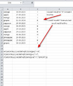
Column A have some Fruits and column B has the month ,
i need Result in "C" column based on the month order, not in fruits order.
for example , first time
i tried "Month formula abut not able to get desired result.
pls some one help me.

Thanks in advance.

 

[madhanji]

Hi, see the linked file for a possible solution...

The formula used in the table...
C1: =IF(A1="","",IF(AND(COUNTIF(A:A,A1)-COUNTIFS(A:A,A1,B:B,">"&B1)>0,COUNTIF(A:A,A1)-COUNTIFS(A:A,A1,B:B,">"&B1)<4),REPT("I",COUNTIF(A:A,A1)-COUNTIFS(A:A,A1,B:B,">"&B1)),"ERROR")) (Range: C1:C25 ...)

FruitsOrder.xlsx

View attachment 90701

View attachment 90702

Dear @fjns sir, S, this formula works perfectly in Office 2010.
( i know/tried with countif function and got how many times repeated fruits came on column A only , I DONT know TO covert this to ....)

A BIG thanks to your contribution

 

[madhanji]

thanks Peter, I wish I could remember where I saw that it was not. I hope a 2010 user will experiment with it for us.

Another page says 2007.

S, ichecked roman function in 2010 and works well

 

[madhanji]

Hi, I created another solution with the ROMAN function also recommended by awoohaw for Office 365.

The formula used in the new table...
C1: =LET(x,COUNTIF(A:A,A1)-COUNTIFS(A:A,A1,B:B,">"&B1),IF(A1="","",IF(x>0,ROMAN(x),""))) (Range: C1:C25 ...)

FruitsOrder2.xlsx

View attachment 90706

View attachment 90707

@fjns , @Peter_SSs LET function not available in 2010 ,Thanks or rewrite , i will try with LET in Higher office VERSION

 

[fjns]

Hi, I am very glad that the formula works.
If I have enough knowledge, I am happy to help at any time.

 

[madhanji]

.. though if that does produce the results that the OP wants, then it would need to be re-written without the LET function as that is definitely not available in 2010 version

Dear @Peter_SSs , can you help me to re-write the below formula for excel 2010 with roman function, excel 2010 supports "Roman" function but not SUPPORT "LET "

C1: =LET(x,COUNTIF(A:A,A1)-COUNTIFS(A:A,A1,B:B,">"&B1),IF(A1="","",IF(x>0,ROMAN(x),"")))

i searched google to Get Addon for LET OF EXCEL 2010 But not available..

 

[fjns]

Hi, the formula of #17 without LET function:

=IF(A1="","",IF(COUNTIF(A:A,A1)-COUNTIFS(A:A,A1,B:B,">"&B1)>0,ROMAN(COUNTIF(A:A,A1)-COUNTIFS(A:A,A1,B:B,">"&B1)),""))

FruitsOrder2WithoutLET.xlsx

 

[Peter_SSs]

Dear @fjns sir, S, this formula works perfectly in Office 2010.

If that formula from post #15 works for you, then does this much simpler one also work for you?
I have included the post #15 formula in column C and my suggestion in column D. In col D I have restricted the range to 1000 rows. You can adjust that to be bigger/smaller but I would avoid using whole column references in a formula like that as the formulas will be considerably slower to calculate with whole column references.

madhanji.xlsm
	A	B	C	D
1	orange	30/10/2023	II	II
2	apple	27/05/2023	I	I
3	mango	30/06/2023	I	I
4	grapes	1/03/2024	II	II
5	pappaya	28/08/2023	I	I
6	orange	30/09/2023	I	I
7	apple	29/10/2023	II	II
8	pappaya	29/11/2023	II	II
9	mango	30/07/2023	II	II
10	pineapple	29/05/2023	I	I
11	pineapple	29/08/2023	II	II
12	grapes	30/12/2023	I	I
Sheet1

Cell Formulas
Range	Formula
C1:C12	C1	=IF(A1="","",IF(AND(COUNTIF(A:A,A1)-COUNTIFS(A:A,A1,B:B,">"&B1)>0,COUNTIF(A:A,A1)-COUNTIFS(A:A,A1,B:B,">"&B1)<4),REPT("I",COUNTIF(A:A,A1)-COUNTIFS(A:A,A1,B:B,">"&B1)),"ERROR"))
D1:D12	D1	=ROMAN(COUNTIFS(A$1:A$1000,A1,B$1:B$1000,"<="&B1))

 

[madhanji]

Hi, the formula of #17 without LET function:

=IF(A1="","",IF(COUNTIF(A:A,A1)-COUNTIFS(A:A,A1,B:B,">"&B1)>0,ROMAN(COUNTIF(A:A,A1)-COUNTIFS(A:A,A1,B:B,">"&B1)),""))

FruitsOrder2WithoutLET.xlsx

Dear ,works perfectly ,,Super

i dont have words

 

[madhanji]

If that formula from post #15 works for you, then does this much simpler one also work for you?
I have included the post #15 formula in column C and my suggestion in column D. In col D I have restricted the range to 1000 rows. You can adjust that to be bigger/smaller but I would avoid using whole column references in a formula like that as the formulas will be considerably slower to calculate with whole column references.

madhanji.xlsm
	A	B	C	D
1	orange	30/10/2023	II	II
2	apple	27/05/2023	I	I
3	mango	30/06/2023	I	I
4	grapes	1/03/2024	II	II
5	pappaya	28/08/2023	I	I
6	orange	30/09/2023	I	I
7	apple	29/10/2023	II	II
8	pappaya	29/11/2023	II	II
9	mango	30/07/2023	II	II
10	pineapple	29/05/2023	I	I
11	pineapple	29/08/2023	II	II
12	grapes	30/12/2023	I	I
Sheet1

Cell Formulas
Range	Formula
C1:C12	C1	=IF(A1="","",IF(AND(COUNTIF(A:A,A1)-COUNTIFS(A:A,A1,B:B,">"&B1)>0,COUNTIF(A:A,A1)-COUNTIFS(A:A,A1,B:B,">"&B1)<4),REPT("I",COUNTIF(A:A,A1)-COUNTIFS(A:A,A1,B:B,">"&B1)),"ERROR"))
D1:D12	D1	=ROMAN(COUNTIFS(A$1:A$1000,A1,B$1:B$1000,"<="&B1))

Dear @Peter_SSs , SORRY ,SORRY , i accidently missed to view /check your formula of "D1" , ITS WORK PERFECTLY ..
Thanks for reminding me and provide the solution ..


Don't mistaken me ,I can't "mark the solution " of #27 th post.. bcas of previous " solution removed"

 

[Peter_SSs]

Thanks for reminding me and provide the solution

You're welcome.

Don't mistaken me ,I can't "mark the solution " of #27 th post.. bcas of previous " solution removed"

Not quite sure what you are saying but you can mark any solution you like, it is up to you. If you change your mind and decide to mark a different solution, the original solution mark will be removed