UDF Count the number of cells coloured by conditional formatting

[Claire Jackson]

I've been searching for days on this and finally have had to ask for help. I can see its been asked many times before but each example I find doesn't work.

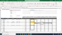
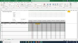
I have a spreadsheet with part of it conditionally formatted with orange based on certain criteria. All I want to do is count the amount of coloured cells and I just can't get it to work.

The cell colour I am looking for is in cell BP1 and the formula in BP2 is this: =@CountConditionColorCells($K$13:$BN$22,BP1)

the code I have is this:

Function COUNTConditionColorCells(CellsRange As Range, ColorRng As Range)
Dim Bambo As Boolean
Dim dbw As String
Dim CFCELL As Range
Dim CF1 As Single
Dim CF2 As Double
Dim CF3 As Long
Bambo = False
For CF1 = 1 To CellsRange.FormatConditions.Count
If CellsRange.FormatConditions(CF1).Interior.ColorIndex = ColorRng.Interior.ColorIndex Then
Bambo = True
Exit For
End If
Next CF1
CF2 = 0
CF3 = 0
If Bambo = True Then
For Each CFCELL In CellsRange
dbw = CFCELL.FormatConditions(CF1).Formula1
dbw = Application.ConvertFormula(dbw, xlA1, xlR1C1)
dbw = Application.ConvertFormula(dbw, xlR1C1, xlA1, , ActiveCell.Resize(CellsRange.Rows.Count, CellsRange.Columns.Count).Cells(CF3 + 1))
If Evaluate(dbw) = True Then CF2 = CF2 + 1
CF3 = CF3 + 1
Next CFCELL
Else
COUNTConditionColorCells = "NO-COLOR"
Exit Function
End If
COUNTConditionColorCells = CF2
End Function

 

[Fluff]

Ok try

=COUNTIFS($B$11:$B$13,$D$2,task_start,"<="&K10,task_end,">="&K10)

The B11:b13 range must be exactly the same size as the two named ranges.

 

[Claire Jackson]

Hi, no sorry that didn't work. I need it to add up all the "orange cells" from the column beneath it based on the lookup trade. e.g. Bricklayer in cell Y13, Y18, Y23 or Joiner in Y14, Y19, Y24 etc.

 

[Fluff]

You will need to change the ranges to suit your sheet.
Also are the actual ranges of the two named ranges?

 

[Claire Jackson]

I don't understand. sorry. Forgetting the trade for now, if I just had a formula that counted all the oranges in the column that would do.

 

[Fluff]

At the moment you are using two named ranges task_start & task_end, which from the image appear to be F2 & G2 which are both empty.
Therefore I don't see how your Cf formula is highlighting anything.

 

[Claire Jackson]

Its only highlighting cells F2 and G2 from your formula above. I want the totals to calculate just from the data from row 13 downwards.

There are 4 orange cells in column Y which I want to be totalled into cell Y2 making cell Y2 show the number 4.
e.g. cell AB2 would show 2 as there are only two orange cells from row 13 downwards.

 

[Fluff]

Its only highlighting cells F2 and G2 from your formula above.

No it's not. Neither F2 nor G2 are mention in the formula.

What exactly are those two named ranges?

 

[Claire Jackson]

Forget the formula it didn't do what I want it to. I just want row 2 to add up the orange cells in row 13 going downwards

 

[Fluff]

I cannot help you until you answer my questions.

 

[Alex Blakenburg]

I think if @Claire Jackson can answer Fluff's question and it can be done by formula then that is the way to go rather than a UDF
Or another option would be to take onboard Mynda Treacy's item 6 "Formatting to Encode Data" in her 10 Things you should never do in Excel, which addresses pretty much this exact issue. It runs from the 7:07 min mark to 8:10. Link below.