52 Week Pivot Table

[DJFANDANGO]

Hi Guys,

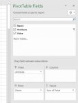
I have a 52 week table with 60 employees, I'd like to put in a Pivot Table that will filter the weeks of the year, that shows how many meetings they've attended, and percentage of the total team.

Is there a way of doing this?

Thanks in advance...

Book1
	A	B	C	D	E	F	G	H	I	J	K	L	M
1	Name	01/01/2020	07/01/2020	13/01/2020	19/01/2020	25/01/2020	31/01/2020	06/02/2020	12/02/2020	18/02/2020	24/02/2020	01/03/2020	07/03/2020
2		wk1	wk2	wk3	wk4	wk5	wk6	wk7	wk8	wk9	wk10	wk11	wk12
3	Sarah	3	0	0	0	2	1	2	2	0	2	0	1
4	John	1	2	0	2	3	0	2	2	1	1	3	1
5	Mike	0	1	2	1	1	1	1	3	1	0	1	2
6	steve	1	0	2	2	3	2	2	0	1	0	1	3
7	Donald	0	2	3	0	0	3	2	1	2	2	1	1
8	Bob	2	2	2	0	2	0	2	1	3	3	1	2
9	Kevin	2	2	3	1	2	3	3	1	3	3	0	0
10	Mandy	2	1	2	2	0	2	2	0	2	2	0	3
11	Susan	0	1	2	3	0	1	2	1	2	2	1	0
12	PERCENTAGE	67%	78%	78%	67%	67%	78%	100%	78%	89%	78%	67%	78%
Sheet1

Cell Formulas
Range	Formula
C1:M1	C1	=B1+6
B12:M12	B12	=COUNTIFS(B3:B11,">=1")/COUNTA(B3:B11)

Named Ranges
Name	Refers To	Cells
Date	=Sheet1!$B$1:$M$1	C1

Cells with Conditional Formatting
Cell	Condition		Cell Format	Stop If True
B12:M12	Other Type	Color scale		NO

 

[DJFANDANGO]

SCRUB the percentage, I don't need that on the pivot table, just a graph chart that shows how many meetings in a given week they attend... I can get the percentage onto another graph... thanks!

 

[alansidman]

Loaded your data into Power Query and unpivoted the data. Here is the Mcode.

let
    Source = Excel.CurrentWorkbook(){[Name="Table1"]}[Content],
    #"Changed Type" = Table.TransformColumnTypes(Source,{{"Column1", type text}, {"wk1", Int64.Type}, {"wk2", Int64.Type}, {"wk3", Int64.Type}, {"wk4", Int64.Type}, {"wk5", Int64.Type}, {"wk6", Int64.Type}, {"wk7", Int64.Type}, {"wk8", Int64.Type}, {"wk9", Int64.Type}, {"wk10", Int64.Type}, {"wk11", Int64.Type}, {"wk12", Int64.Type}}),
    #"Renamed Columns" = Table.RenameColumns(#"Changed Type",{{"Column1", "Name"}}),
    #"Unpivoted Other Columns" = Table.UnpivotOtherColumns(#"Renamed Columns", {"Name"}, "Attribute", "Value")
in
    #"Unpivoted Other Columns"

Then in Excel created a Pivot Table.

Book3
	A	B	C	D	E	F	G
1	Name	Attribute	Value		Attribute	wk1
2	Sarah	wk1	3
3	Sarah	wk2	0		Name	Sum of Value
4	Sarah	wk3	0		Bob	2
5	Sarah	wk4	0		Donald	0
6	Sarah	wk5	2		John	1
7	Sarah	wk6	1		Kevin	2
8	Sarah	wk7	2		Mandy	2
9	Sarah	wk8	2		Mike	0
10	Sarah	wk9	0		Sarah	3
11	Sarah	wk10	2		steve	1
12	Sarah	wk11	0		Susan	0
13	Sarah	wk12	1
14	John	wk1	1
15	John	wk2	2
16	John	wk3	0
17	John	wk4	2
18	John	wk5	3
19	John	wk6	0
20	John	wk7	2
21	John	wk8	2
22	John	wk9	1
23	John	wk10	1
24	John	wk11	3
25	John	wk12	1
26	Mike	wk1	0
27	Mike	wk2	1
28	Mike	wk3	2
29	Mike	wk4	1
30	Mike	wk5	1
31	Mike	wk6	1
32	Mike	wk7	1
33	Mike	wk8	3
34	Mike	wk9	1
35	Mike	wk10	0
36	Mike	wk11	1
37	Mike	wk12	2
38	steve	wk1	1
39	steve	wk2	0
40	steve	wk3	2
41	steve	wk4	2
42	steve	wk5	3
43	steve	wk6	2
44	steve	wk7	2
45	steve	wk8	0
46	steve	wk9	1
47	steve	wk10	0
48	steve	wk11	1
49	steve	wk12	3
50	Donald	wk1	0
51	Donald	wk2	2
52	Donald	wk3	3
53	Donald	wk4	0
54	Donald	wk5	0
55	Donald	wk6	3
56	Donald	wk7	2
57	Donald	wk8	1
58	Donald	wk9	2
59	Donald	wk10	2
60	Donald	wk11	1
61	Donald	wk12	1
62	Bob	wk1	2
63	Bob	wk2	2
64	Bob	wk3	2
65	Bob	wk4	0
66	Bob	wk5	2
67	Bob	wk6	0
68	Bob	wk7	2
69	Bob	wk8	1
70	Bob	wk9	3
71	Bob	wk10	3
72	Bob	wk11	1
73	Bob	wk12	2
74	Kevin	wk1	2
75	Kevin	wk2	2
76	Kevin	wk3	3
77	Kevin	wk4	1
78	Kevin	wk5	2
79	Kevin	wk6	3
80	Kevin	wk7	3
81	Kevin	wk8	1
82	Kevin	wk9	3
83	Kevin	wk10	3
84	Kevin	wk11	0
85	Kevin	wk12	0
86	Mandy	wk1	2
87	Mandy	wk2	1
88	Mandy	wk3	2
89	Mandy	wk4	2
90	Mandy	wk5	0
91	Mandy	wk6	2
92	Mandy	wk7	2
93	Mandy	wk8	0
94	Mandy	wk9	2
95	Mandy	wk10	2
96	Mandy	wk11	0
97	Mandy	wk12	3
98	Susan	wk1	0
99	Susan	wk2	1
100	Susan	wk3	2
101	Susan	wk4	3
102	Susan	wk5	0
103	Susan	wk6	1
104	Susan	wk7	2
105	Susan	wk8	1
106	Susan	wk9	2
107	Susan	wk10	2
108	Susan	wk11	1
109	Susan	wk12	0
Sheet2

 

[DJFANDANGO]

Thanks for the info Alan, unfortunately, I have never used Power Query before, wouldn't know where to start...?

 

[alansidman]

Click on the link in my signature block to get started. If truly interested in learning PQ, then obtain "M is for (Data) Monkey" by Ken Puls and Miguel Escobar. Available on MR. E Sore or Amazon.

Products

Products / books about Microsoft Excel.

www.mrexcel.com

 

[alansidman]

Thanks for the info Alan, unfortunately, I have never used Power Query before, wouldn't know where to start...?

Here are the steps I used.
1. Highlight your table in Excel
2. Click on the Data Tab. Select Get from Table/Range on the Get and Transform section
3. In the PQ editor Right Click on Column 1 and select Rename. Rename "Name"
4. Highlight Name Column and click on Transform Tab. Select Unpivot and then Unpivot Other Columns
5. On the Home Tab. Click on Close and Load.
You now have a list that you can use to create a Pivot Table back in Native Excel.