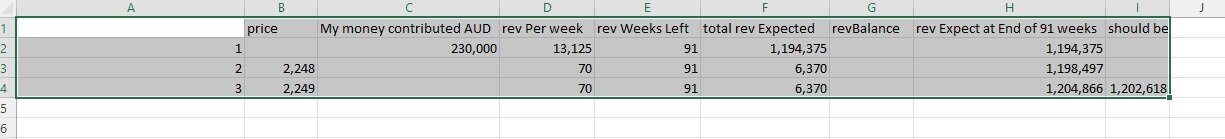
hi everyone this is stumping me so have this table below and trying to work out column H and G. Column H in in H3 i am trying to add H2 plus F2 + F3 minus B3 and get a result and then H4 i am trying to add F2+F3=F4 minus B3 and B4 and so on. so i have this formula for H3 =SUM(F$2:F3)-@B$3:B3 and it works for that cell but when i copy it down it does not work.
the second part is column G i am trying to work out running balance of rev per week as D column numbers are paid each week so for instance last week i got 13,125 from revenue in column A and no week 2 i get another 13,125 (A1) plus 70 from A2 and 70 from A3 to i should have a balance and then i take some of that revenue and buy another item in A4 which is 2,500 and get 80 per week so the balance should come down but the revenue goes up
appreciate your help
| Book1.xlsx | |||||||||||
|---|---|---|---|---|---|---|---|---|---|---|---|
| A | B | C | D | E | F | G | H | I | |||
| 1 | price | My money contributed AUD | rev Per week | rev Weeks Left | total rev Expected | revBalance | rev Expect at End of 91 weeks | should be | |||
| 2 | 1 | 230,000 | 13,125 | 91 | 1,194,375 | 1,194,375 | |||||
| 3 | 2 | 2,248 | 70 | 91 | 6,370 | 1,198,497 | |||||
| 4 | 3 | 2,249 | 70 | 91 | 6,370 | 1,204,866 | 1,202,618 | ||||
| 5 | |||||||||||
| 6 | |||||||||||
| 7 | |||||||||||
| 8 | |||||||||||
| 9 | |||||||||||
| 10 | |||||||||||
| 11 | |||||||||||
Sheet1 | |||||||||||
| Cell Formulas | ||
|---|---|---|
| Range | Formula | |
| F2:F4 | F2 | =SUM(D2*E2) |
| H2 | H2 | =SUM(F$2:F2) |
| H3:H4 | H3 | =@SUM(F$2:F3)-@B$3:B3 |