Age calculation in Text Format, in year, month and day.

[harzer]

I am facing a problem despite my research on the net, I confess that I can not find it.
Namely that I am unable to handle array variables correctly, which complicates my task.

I have a large amount of row data, in 10 columns, the ones that concern the present case, are columns E and H.
for now, column E is empty.
Column H contains dates of birth.
How to proceed, either by table or table combined with dictionary to indicate the age in: year, month and days in column E, according to the current date.
The goal is to have the result in text format, (Example: 15y 5m 10d), I thought of making a call to a function which would give the result just in text so as not to use formulas (No formulas) Please .
Unless I am mistaken, the desired result for the first 10 lines is in column L, based on the date that the calculation was made is: 30-01-2023
Thank you very much in advance for your suggestions.
PS: I completely emptied my table and I simply left the two columns concerned so that you can (eventually) test your code.

CalculAge1.xlsm
	A	B	C	D	E	F	G	H	I	J	K	L	M
1					Age			Né(e)				Age
2								16-03-1957				65 a 10 m 14 j
3								17-04-2012				10 a 9 m 13 j
4								14-04-2012				10 a 9 m 16 j
5								25-03-1966				56 a 10 m 5 j
6								30-05-1959				63 a 8 m 0 j
7								17-02-1962				60 a 11 m 13 j
8								22-01-1955				68 a 0 m 8 j
9								15-02-1961				61 a 11 m 15 j
10								18-04-2012				10 a 9 m 12 j
11								1-01-2010				13 a 0 m 29 j
12								22-03-2019
13								15-04-2007
14								15-04-2007
15								15-04-2007
16								16-04-2007
17								15-04-2008
18								15-04-2008
19								15-04-2008
20								15-04-2008
21								15-04-2008
22								15-04-2008
23								15-04-2008
24								15-05-2008
25								15-04-2008
Parents

 

[James006]

Hi,

You can test
=DATEDIF(H2,TODAY(),"y")&" a "&DATEDIF(H2,TODAY(),"ym")&" m "&DATEDIF(H2,TODAY(),"yd")&" j "

 

[James006]

Hi again,

From your comment, it would appear you need an UDF for the complete Age ...

Function Age(rng As Range)
' Dans la cellule L2 saisir = age(H2)
  Age = Evaluate("=DATEDIF(" & CLng(rng.Value) & ",TODAY(),""y"")&"" a ""&DATEDIF(" & CLng(rng.Value) & ",TODAY(),""ym"")&"" m ""&DATEDIF(" & CLng(rng.Value) & ",TODAY(),""yd"")&"" j """)
End Function

 

[Z51]

If you truly don't want a formula in the cells in column E, you can use Evaluate in VBA to produce the same results as the DATEDIF worksheet function, e.g.

Sub harzer()
Dim i As Long, lastrow As Long
lastrow = Range("H" & Rows.Count).End(xlUp).Row

For i = 2 To lastrow
    Cells(i, 5).Value = _
        Evaluate("DATEDIF(""" & Cells(i, 8).Value & """,""" & Date & """,""Y"")") & " y " & _
        Evaluate("DATEDIF(""" & Cells(i, 8).Value & """,""" & Date & """,""YM"")") & " m " & _
        Evaluate("DATEDIF(""" & Cells(i, 8).Value & """,""" & Date & """,""MD"")") & " d"
Next i
End Sub

You could adjust this code to go in the Worksheet_Change event, so it gets triggered anytime you enter a value in column H. If you ran the code above, it would generate the age for all values in column H into column E. You may also want to account for adjusting the values when opening the workbook (in the Workbook_Open event) so that it's always current.

 

[harzer]

Hello
I am very happy that you have understood my request, I was afraid of not explaining the problem well.
Thank you for your quick response, however, as my file is very very heavy, I took the liberty of asking you to avoid formulas which only make the execution of my Marcos heavier and above all slow down.
Can you (please) try using arrays instead of formulas.
I know it will take longer to code, it will be the challenge for connoisseurs like you to help novices like me.
Thank you so much.

 

[Z51]

See my post for direct VBA (no formulas).

 

[harzer]

Hello Z51,
Thank you for your reply.
I tested your code but unfortunately I got runtime error '13' type mismatch.

 

[harzer]

Hello James006,
I am answering to tell you that there is a problem with the number of days. for example for the date of 16-03-1957, I must have: 65 a 10 m 14 d but I have: 65 a 10 m 320 d .
Thank you so much.

 

[Z51]

Make sure your "dates" in column H are actual dates and not text representations of dates. If you format the cells as numbers they should show you 5-digit numeric values probably in the range of 18264 to 44956, which are Jan 1, 1950 to today.

My code works fine for me as provided (against your data that I copied from your original post). I added the CLng function below, like James used in his code, but don't see why that would make any difference. They both work the same.

Sub harzer()
Dim i As Long, lastrow As Long
lastrow = Range("H" & Rows.Count).End(xlUp).Row

For i = 2 To lastrow
    Cells(i, 5).Value = _
        Evaluate("DATEDIF(""" & CLng(Cells(i, 8).Value) & """,""" & Date & """,""Y"")") & " y " & _
        Evaluate("DATEDIF(""" & CLng(Cells(i, 8).Value) & """,""" & Date & """,""YM"")") & " m " & _
        Evaluate("DATEDIF(""" & CLng(Cells(i, 8).Value) & """,""" & Date & """,""MD"")") & " d"
Next i
End Sub

 

[harzer]

Hello Z51,
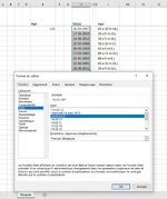
I'm sorry but I still have the same error and yet my column H and in date format, see attached photo, Do you want me to send you my little file as an attachment to your address?
For your information, I must inform you that I have the version of Excel 2016 French version. Would there be a conflict at this level?