Automate task in vba

[plutonik33]

Hi,

I don't have vba experience, but I really need to solve the following tasks:

First table has to be filtered by unique users.
Filtered table then needs to be stored in a new document and named after the name of the user.

Plus it would be amazing if I can then send the generated documents attached as an email with subject text and additional information like "Dear User, ...." (Using Outlook).

Appreciate any help!

Here is my Mini-sheet:

Filter by column 'User'.xlsx
	A	B	C	D	E	F	G	H	I	J	K	L	M	N	O	P	Q	R	S	T	U	V
1	Reihenfolge	EndSZ	SM-Auftrags-nummer	Position für Google Maps	Straße	PLZ	Ort	Prio	Tausch gegen	ON	ONKZ	AsB	Region_PTI	Material-nummer	Jahr	Kalender-woche	Wartungs-fenster	User	Wartungs-fenster Datum	Beginn Wartungs-fenster	Ende Wartungs-fenster	IP
2	xx	xx	xx	xx	xx	xx	xx	xx	xx	xx	xx	xx	xx	xx	xx	xx	xx	S1	xx	xx	xx	xx
3	xx	xx	xx	xx	xx	xx	xx	xx	xx	xx	xx	xx	xx	xx	xx	xx	xx	S1	xx	xx	xx	xx
4	xx	xx	xx	xx	xx	xx	xx	xx	xx	xx	xx	xx	xx	xx	xx	xx	xx	S2	xx	xx	xx	xx
5	xx	xx	xx	xx	xx	xx	xx	xx	xx	xx	xx	xx	xx	xx	xx	xx	xx	S2	xx	xx	xx	xx
6	xx	xx	xx	xx	xx	xx	xx	xx	xx	xx	xx	xx	xx	xx	xx	xx	xx	S3	xx	xx	xx	xx
7	xx	xx	xx	xx	xx	xx	xx	xx	xx	xx	xx	xx	xx	xx	xx	xx	xx	S3	xx	xx	xx	xx
8	xx	xx	xx	xx	xx	xx	xx	xx	xx	xx	xx	xx	xx	xx	xx	xx	xx	S4	xx	xx	xx	xx
9	xx	xx	xx	xx	xx	xx	xx	xx	xx	xx	xx	xx	xx	xx	xx	xx	xx	S4	xx	xx	xx	xx
Tabelle2

Cells with Conditional Formatting
Cell	Condition		Cell Format	Stop If True
A2:A9	Expression	=#BEZUG!="nein"	text	NO
H2:H9	Cell Value	="entfällt"	text	NO
H2:H9	Cell Value	="entfällt"	text	NO
B2:V9	Expression	=#BEZUG!="nein"	text	NO
B1	Cell Value	duplicates	text	NO

 

[mumps]

What would you like to enter as the subject text and additional information? Is the email address anywhere in your data? It would be helpful if you could post an English version to help us better understand the headers.

 

[plutonik33]

Hi mumps,

thank you for the quick reply! Is it possible to leave the headers as they are? Only relevant ones are 'User', 'Email' (I will add this column right next to 'User'), 'Name' (full name of user) and 'week'.

As Subject text: "Operational plan for " 'User' "-" 'Name' "-" 'Week'
Additional Information: "Dear" 'Name' ",enclosed is the operational plan for" 'Week' "."


Here the updated Minisheet (relevant columns are merked green):

Filter by column 'User'.xlsx
	A	B	C	D	E	F	G	H	I	J	K	L	M	N	O	P	Q	R	S	T	U	V	W	X
2	xx	xx	xx	xx	xx	xx	xx	xx	xx	xx	xx	xx	xx	xx	xx	week1	xx	S1	user1@hotmail.com	Max Mustermann	xx	xx	xx	xx
3	xx	xx	xx	xx	xx	xx	xx	xx	xx	xx	xx	xx	xx	xx	xx	week1	xx	S1	user1@hotmail.com	Max Mustermann	xx	xx	xx	xx
4	xx	xx	xx	xx	xx	xx	xx	xx	xx	xx	xx	xx	xx	xx	xx	week2	xx	S2	user2@hotmail.com	Peter Mustermann	xx	xx	xx	xx
5	xx	xx	xx	xx	xx	xx	xx	xx	xx	xx	xx	xx	xx	xx	xx	week2	xx	S2	user2@hotmail.com	Peter Mustermann	xx	xx	xx	xx
6	xx	xx	xx	xx	xx	xx	xx	xx	xx	xx	xx	xx	xx	xx	xx	week3	xx	S3	user3@hotmail.com	Greta Mustermann	xx	xx	xx	xx
7	xx	xx	xx	xx	xx	xx	xx	xx	xx	xx	xx	xx	xx	xx	xx	week3	xx	S3	user3@hotmail.com	Greta Mustermann	xx	xx	xx	xx
8	xx	xx	xx	xx	xx	xx	xx	xx	xx	xx	xx	xx	xx	xx	xx	week4	xx	S4	user4@hotmail.com	Timo Mustermann	xx	xx	xx	xx
9	xx	xx	xx	xx	xx	xx	xx	xx	xx	xx	xx	xx	xx	xx	xx	week4	xx	S4	user4@hotmail.com	Timo Mustermann	xx	xx	xx	xx
Tabelle2

Cells with Conditional Formatting
Cell	Condition		Cell Format	Stop If True
A2:A9	Expression	=#BEZUG!="nein"	text	NO
H2:H9	Cell Value	="entfällt"	text	NO
H2:H9	Cell Value	="entfällt"	text	NO
B2:X9	Expression	=#BEZUG!="nein"	text	NO

 

[plutonik33]

Filter by column 'User'.xlsx
	A	B	C	D	E	F	G	H	I	J	K	L	M	N	O	P	Q	R	S	T	U	V	W	X
1	Reihenfolge	EndSZ	SM-Auftrags-nummer	Position für Google Maps	Straße	PLZ	Ort	Prio	Tausch gegen	ON	ONKZ	AsB	Region_PTI	Material-nummer	Jahr	Week	Wartungs-fenster	User	Email	Name	Wartungs-fenster Datum	Beginn Wartungs-fenster	Ende Wartungs-fenster	IP
2	xx	xx	xx	xx	xx	xx	xx	xx	xx	xx	xx	xx	xx	xx	xx	week1	xx	S1	user1@hotmail.com	Max Mustermann	xx	xx	xx	xx
3	xx	xx	xx	xx	xx	xx	xx	xx	xx	xx	xx	xx	xx	xx	xx	week1	xx	S1	user1@hotmail.com	Max Mustermann	xx	xx	xx	xx
4	xx	xx	xx	xx	xx	xx	xx	xx	xx	xx	xx	xx	xx	xx	xx	week2	xx	S2	user2@hotmail.com	Peter Mustermann	xx	xx	xx	xx
5	xx	xx	xx	xx	xx	xx	xx	xx	xx	xx	xx	xx	xx	xx	xx	week2	xx	S2	user2@hotmail.com	Peter Mustermann	xx	xx	xx	xx
6	xx	xx	xx	xx	xx	xx	xx	xx	xx	xx	xx	xx	xx	xx	xx	week3	xx	S3	user3@hotmail.com	Greta Mustermann	xx	xx	xx	xx
7	xx	xx	xx	xx	xx	xx	xx	xx	xx	xx	xx	xx	xx	xx	xx	week3	xx	S3	user3@hotmail.com	Greta Mustermann	xx	xx	xx	xx
8	xx	xx	xx	xx	xx	xx	xx	xx	xx	xx	xx	xx	xx	xx	xx	week4	xx	S4	user4@hotmail.com	Timo Mustermann	xx	xx	xx	xx
9	xx	xx	xx	xx	xx	xx	xx	xx	xx	xx	xx	xx	xx	xx	xx	week4	xx	S4	user4@hotmail.com	Timo Mustermann	xx	xx	xx	xx
Tabelle2

Cells with Conditional Formatting
Cell	Condition		Cell Format	Stop If True
A2:A9	Expression	=#BEZUG!="nein"	text	NO
H2:H9	Cell Value	="entfällt"	text	NO
H2:H9	Cell Value	="entfällt"	text	NO
B2:X9	Expression	=#BEZUG!="nein"	text	NO
B1	Cell Value	duplicates	text	NO

 

[mumps]

In order to re-name the new workbooks, they have to be saved. What is the full path to the folder where you want to save the new workbooks?

 

[plutonik33]

In order to re-name the new workbooks, they have to be saved. What is the full path to the folder where you want to save the new workbooks?

For now it would be perfect if I can save the generated documents in following path "C:\Users\Documents\Tauschprojekt"

 

[mumps]

Try:

Sub CreateEmails()
    Application.ScreenUpdating = False
    Dim v As Variant, i As Long, dic As Object, srcWB As Workbook, srcWS As Worksheet
    Dim OutApp As Object, OutMail As Object
    Set srcWB = ThisWorkbook
    Set srcWS = srcWB.Sheets(1)
    With srcWS
        v = .Range("R2", .Range("R" & .Rows.Count).End(xlUp)).Value
    End With
    Set dic = CreateObject("Scripting.Dictionary")
    Set OutApp = CreateObject("Outlook.Application")
    For i = 1 To UBound(v, 1)
        If Not dic.Exists(v(i, 1)) Then
            dic.Add v(i, 1), Nothing
            With srcWS
                .Range("A1").CurrentRegion.AutoFilter 18, v(i, 1)
                .AutoFilter.Range.Copy
                Workbooks.Add 1
                Range("A1").PasteSpecial
                ActiveWorkbook.SaveAs Filename:="C:\Users\Documents\Tauschprojekt\" & Range("R2") & ".xlsx", FileFormat:=51
                Set OutMail = OutApp.CreateItem(0)
                With OutMail
                    .To = Range("S2").Value
                    .Subject = "Operational plan for " & Range("S2").Value & "-" & Range("T2").Value & "-" & Range("P2").Value
                    .HTMLBody = "Dear " & Range("T2").Value & "," & "<br><br>" & "Enclosed is the operational plan for " & Range("P2").Value & "."
                    .attachments.Add ActiveWorkbook.FullName
                    .Display
                End With
                ActiveWorkbook.Close False
            End With
        End If
    Next i
    srcWS.Range("A1").AutoFilter
    Application.ScreenUpdating = True
End Sub

 

[plutonik33]

You are my hero!!! Thank you for this noble-minded effort

 

[mumps]

You are very welcome.

 

[plutonik33]

Hi,

my next task is very specific and I am struggling with it, because connected cells and a special paste is involved. Also because I lack vba experience.
Hope you can help...

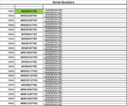
Short Version: I have two documents and I want to copy serial numbers from one document and paste in another document with connected cells.

Detailed explanation:

1) Copy Range("A1:B1) from source "document1.xlsm" to a temporary document "temp.xlsx" in Range("A1:B1") -> Now I have the headers in "temp.xlsx".
2) Copy Range("A2:B8") from source "document1.xlsm" and paste in "temp.xlsx" underneath the headers in Range("A2:B8") and format Range("A1:B8") as a table. -> Now I have the first half of my table
3) In "temp.xlsx" copy Range("A2:B8") and paste it in underneath in Range("A9:B15") -> This is an intermediary step because I need redundant data in order to be able to paste in connected cells later on.
4) Now I sort this table by increasing number in column 'Order'


The result should look like this:

Order SerialNumber
1 49/6353/5/71E2
1 49/6353/5/71E2
2 49/6322/54/71E1
2 49/6322/54/71E1
3 49/6322/53/71E1
3 49/6322/53/71E1
4 49/6322/51/71E1
4 49/6322/51/71E1
5 49/6322/52/71E1
5 49/6322/52/71E1
6 49/6395/4/71E2
6 49/6395/4/71E2
7 49/6393/6/71E2
7 49/6393/6/71E2


This copy and paste mechanism has to be repeated for all Ranges of the table where number starts at 1 and ends one row before next number 1 starts.
To better understand what I mean, needed Ranges are seperated by thik lines.

As a result these additional tables:

Order SerialNumber
1 49/6307/9/71E2
1 49/6307/9/71E2
2 49/6307/8/71E2
2 49/6307/8/71E2
3 49/631/663/71E1
3 49/631/663/71E1
4 49/6352/33/71E2
4 49/6352/33/71E2
5 49/6353/4/71E2
5 49/6353/4/71E2
6 49/6353/9/71E2
6 49/6353/9/71E2
7 49/6353/11/71E2
7 49/6353/11/71E2
8 49/6353/13/71E2
8 49/6353/13/71E2

And

Order SerialNumber
1 49/6335/13/71EA
1 49/6335/13/71EA
2 49/6335/9/71EA
2 49/6335/9/71EA
3 49/681/854/71E2
3 49/681/854/71E2
4 49/681/235/71E2
4 49/681/235/71E2
5 49/681/922/71E2
5 49/681/922/71E2
6 49/681/252/71E2
6 49/681/252/71E2


Now that I have my tables with redundant sorted data prepared in "temp.xlsx", I have to copy the sorted Ranges one by one into "document2.xlsx"

1) Copy first sorted Range("B2:B15") and paste as formula (I have to do this because of connected cells) in connected Cell("B4:B5") (I marked this cell in green in "document2.xlsx")
2) Copy second sorted Range and paste underneath in "document2.xlsx" and so on...


The result should look like attached image "document2_result.PNG"

I hope you can follow my explanation and it would be amazing if you can help me once more!

------------------------------------------------------------------------------------------------------------
1) "document1.xlsm"

document1.xlsx
	A	B
1	Order	SerialNumber
2	1	49/6353/5/71E2
3	2	49/6322/54/71E1
4	3	49/6322/53/71E1
5	4	49/6322/51/71E1
6	5	49/6322/52/71E1
7	6	49/6395/4/71E2
8	7	49/6393/6/71E2
9	1	49/6307/9/71E2
10	2	49/6307/8/71E2
11	3	49/631/663/71E1
12	4	49/6352/33/71E2
13	5	49/6353/4/71E2
14	6	49/6353/9/71E2
15	7	49/6353/11/71E2
16	8	49/6353/13/71E2
17	1	49/6335/13/71EA
18	2	49/6335/9/71EA
19	3	49/681/854/71E2
20	4	49/681/235/71E2
21	5	49/681/922/71E2
22	6	49/681/252/71E2
Source

Cells with Conditional Formatting
Cell	Condition		Cell Format	Stop If True
B17:B22	Expression	=#BEZUG!="nein"	text	NO
B9:B16	Expression	=#BEZUG!="nein"	text	NO
B2:B8	Expression	=#BEZUG!="nein"	text	NO
B1	Cell Value	duplicates	text	NO

2) "document2.xlsm"

document2.xlsx
	A	B	C	D
1	Serial Numbers
2
3
4	ENDSZ:		Serial Nummer alt:
5			Serial Nummer neu:
6	ENDSZ:		Serial Nummer alt:
7			Serial Nummer neu:
8	ENDSZ:		Serial Nummer alt:
9			Serial Nummer neu:
10	ENDSZ:		Serial Nummer alt:
11			Serial Nummer neu:
12	ENDSZ:		Serial Nummer alt:
13			Serial Nummer neu:
14	ENDSZ:		Serial Nummer alt:
15			Serial Nummer neu:
16	ENDSZ:		Serial Nummer alt:
17			Serial Nummer neu:
18	ENDSZ:		Serial Nummer alt:
19			Serial Nummer neu:
20	ENDSZ:		Serial Nummer alt:
21			Serial Nummer neu:
22	ENDSZ:		Serial Nummer alt:
23			Serial Nummer neu:
24	ENDSZ:		Serial Nummer alt:
25			Serial Nummer neu:
26	ENDSZ:		Serial Nummer alt:
27			Serial Nummer neu:
28	ENDSZ:		Serial Nummer alt:
29			Serial Nummer neu:
30	ENDSZ:		Serial Nummer alt:
31			Serial Nummer neu:
32	ENDSZ:		Serial Nummer alt:
33			Serial Nummer neu:
34	ENDSZ:		Serial Nummer alt:
35			Serial Nummer neu:
36	ENDSZ:		Serial Nummer alt:
37			Serial Nummer neu:
38	ENDSZ:		Serial Nummer alt:
39			Serial Nummer neu:
40	ENDSZ:		Serial Nummer alt:
41			Serial Nummer neu:
42	ENDSZ:		Serial Nummer alt:
43			Serial Nummer neu:
44	ENDSZ:		Serial Nummer alt:
45			Serial Nummer neu:
46	ENDSZ:		Serial Nummer alt:
47			Serial Nummer neu:
48	ENDSZ:		Serial Nummer alt:
49			Serial Nummer neu:
50	ENDSZ:		Serial Nummer alt:
51			Serial Nummer neu:
52	ENDSZ:		Serial Nummer alt:
53			Serial Nummer neu:
54	ENDSZ:		Serial Nummer alt:
55			Serial Nummer neu:
56	ENDSZ:		Serial Nummer alt:
57			Serial Nummer neu:
58	ENDSZ:		Serial Nummer alt:
59			Serial Nummer neu:
60	ENDSZ:		Serial Nummer alt:
61			Serial Nummer neu:
62	ENDSZ:		Serial Nummer alt:
63			Serial Nummer neu:
64	ENDSZ:		Serial Nummer alt:
65			Serial Nummer neu:
66	ENDSZ:		Serial Nummer alt:
67			Serial Nummer neu:
Seriennummer