Setup:
I am trying to set up a very simple end of day cash balance report. Fact table will be a list of all bank accounts and the end of day cash balance. I have lookup tables keyed on account number to link things like Bank Name, Country, and Department.
Problem:
Over the course of the year, any single account may be moved from department to department. So, account 1111 might be in Department A for 1/1/2020 - 5/15/2020, and then moved to Department B for 5/16/2020-onward.
For my visuals, the user will be selecting a single date from a SLICER .
I want to make sure that when a date is picked, the Account's cash balance is included in the correct Department, but I am having trouble with writing that measure (or calculated column if that is best).
What is best practice for setting something like this up with effective dates? Thanks so much!
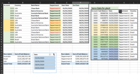
Example of Lookup table:
Fact table:
Example of visuals....

I am trying to set up a very simple end of day cash balance report. Fact table will be a list of all bank accounts and the end of day cash balance. I have lookup tables keyed on account number to link things like Bank Name, Country, and Department.
Problem:
Over the course of the year, any single account may be moved from department to department. So, account 1111 might be in Department A for 1/1/2020 - 5/15/2020, and then moved to Department B for 5/16/2020-onward.
For my visuals, the user will be selecting a single date from a SLICER .
I want to make sure that when a date is picked, the Account's cash balance is included in the correct Department, but I am having trouble with writing that measure (or calculated column if that is best).
What is best practice for setting something like this up with effective dates? Thanks so much!
Example of Lookup table:
| Test for May.xlsx | ||||||||
|---|---|---|---|---|---|---|---|---|
| A | B | C | D | E | F | |||
| 1 | Account Number | Country | Bank Name | Department | Department Start Date | Department End Date | ||
| 2 | 1111 | USA | Chase Bank | Department A | 1/1/2020 | 6/30/2020 | ||
| 3 | 2222 | USA | Bank of America | Department A | 1/1/2020 | |||
| 4 | 3333 | Australia | Australia National Bank | Department A | 1/1/2020 | |||
| 5 | 4444 | Brazil | Brazil Bank | Department A | 1/1/2020 | |||
| 6 | 5555 | Australia | Australia National Bank | Department B | 1/1/2020 | |||
| 7 | 6666 | Canada | Canada First Bank | Department B | 1/1/2020 | |||
| 8 | 7777 | Canada | Canada First Bank | Department B | 1/1/2020 | |||
| 9 | 8888 | UK | Royal Bank | Department C | 1/1/2020 | |||
| 10 | 9999 | USA | JP Morgan | Department C | 1/1/2020 | |||
| 11 | 1111 | USA | Chase Bank | Department B | 7/1/2020 | |||
Sheet1 | ||||||||
Fact table:
| Test for May.xlsx | |||||
|---|---|---|---|---|---|
| A | B | C | |||
| 1 | Account Number | Cash Balance | Date | ||
| 2 | 1111 | $ 49,433,729.00 | 1/1/2020 | ||
| 3 | 2222 | $ 43,764,083.00 | 1/1/2020 | ||
| 4 | 3333 | $ 25,655,834.00 | 1/1/2020 | ||
| 5 | 4444 | $ 3,078,702.00 | 1/1/2020 | ||
| 6 | 5555 | $ 9,520,004.00 | 1/1/2020 | ||
| 7 | 6666 | $ 15,658,861.00 | 1/1/2020 | ||
| 8 | 7777 | $ 31,283,507.00 | 1/1/2020 | ||
| 9 | 8888 | $ 48,068,531.00 | 1/1/2020 | ||
| 10 | 9999 | $ 36,436,769.00 | 1/1/2020 | ||
| 11 | 1111 | $ 38,056,864.00 | 1/2/2020 | ||
| 12 | 2222 | $ 1,229,319.00 | 1/2/2020 | ||
| 13 | 3333 | $ 6,587,544.00 | 1/2/2020 | ||
| 14 | 4444 | $ 41,818,337.00 | 1/2/2020 | ||
| 15 | 5555 | $ 9,010,454.00 | 1/2/2020 | ||
| 16 | 6666 | $ 42,345,150.00 | 1/2/2020 | ||
| 17 | 7777 | $ 23,146,931.00 | 1/2/2020 | ||
| 18 | 8888 | $ 47,767,511.00 | 1/2/2020 | ||
| 19 | 9999 | $ 9,722,558.00 | 1/2/2020 | ||
| 20 | 1111 | $ 17,657,590.00 | 1/3/2020 | ||
| 21 | 2222 | $ 50,448,822.00 | 1/3/2020 | ||
| 22 | { and so on and so on} | ||||
Sheet2 | |||||
| Cell Formulas | ||
|---|---|---|
| Range | Formula | |
| B2:B21 | B2 | =RANDBETWEEN(0,55000000) |
Example of visuals....