Basic Conditional Formatting...

[RandyD123]

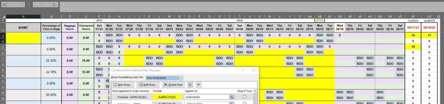
I just want to make each name cell in A turn yellow if either cell in LP or LQ 3 and 4 are over 13.... When I try to select a range it highlights all of the cells in A. They have to work independently of each other. Not sure what I am doing wrong?

Example: Any cell in LP3, LP4, LQ3, LQ4 is over 13 then A3 has to turn yellow. Then if LP5, LP6, LQ5, LQ6 is over 13, then A5 has to turn yellow..... and so on.

 

[RandyD123]

Sorry forgot to upload example.

 

[Joe4]

Your image kind of makes my question your original requirements. I am a bit confused regarding the relationships between columns A, LP, and LQ.
In your description, you mention cells A3 and then A5 skipping over A4. But in your image, A4 is shown as yellow.

So, does every row in column A look at only the SAME rows for LP and LQ?

Or should it skip rows in column A, so that:
A3 looks at LP3:LQ4
A5 looks at LP5:LQ6
A7 looks at LP7:LQ8
etc.

 

[Toadstool]

Hi RandyD123,

Does this work for you?

RandyD123.xlsx
	A	B																																																																																																																																																																																																																																																																																																																																					LO	LP	LQ
1	Column A																																																																																																																																																																																																																																																																																																																																							Column LP	Column LQ
2	Row 2
3	Row 3																																																																																																																																																																																																																																																																																																																																							1	2
4	Row 4																																																																																																																																																																																																																																																																																																																																							3	4
5	Row 5																																																																																																																																																																																																																																																																																																																																							11	12
6	Row 6																																																																																																																																																																																																																																																																																																																																							13	14
7	Row 7																																																																																																																																																																																																																																																																																																																																							14	2
8	Row 8																																																																																																																																																																																																																																																																																																																																							2	2
9	Row 9																																																																																																																																																																																																																																																																																																																																							7	7
Sheet1

Cell Formulas
Range	Formula
A2:A9	A2	="Row "&ROW()

Cells with Conditional Formatting
Cell	Condition		Cell Format	Stop If True
A3:A31	Expression	=AND(ISODD(ROW()),OR(LP3>13,LQ3>13,LP4>13,LQ4>13))	text	NO

 

[RandyD123]

My A column is a range of A3:A104. Everyone has a merged cell in the A column. It corresponds to the LP and LQ column. How ever LP and LQ are simply a count of consecutive zeros. And that person in the A column can only be in one of two places, that why they have two rows.

 

[RandyD123]

Your image kind of makes my question your original requirements. I am a bit confused regarding the relationships between columns A, LP, and LQ.
In your description, you mention cells A3 and then A5 skipping over A4. But in your image, A4 is shown as yellow.

So, does every row in column A look at only the SAME rows for LP and LQ?

Or should it skip rows in column A, so that:
A3 looks at LP3:LQ4
A5 looks at LP5:LQ6
A7 looks at LP7:LQ8
etc.

Yes I believe that is correct. If you notice that each person can be in one of two locations on any given day. They actually can be in both locations on the same day. The LP and LQ columns only count consecutive zeros. I can probably eliminate the LP column, it is being used for testing right now because the consecutive zero thing is broken.

 

[Joe4]

OK, did you look at Toadstool's reply?
I think his solution will do what you want.

Also, I would caution you about using merged cells. They are quite possibly the worst thing in Excel, and can cause all sorts of issues for VBA and things like sorting.
Because of all the potential headaches they can cause, most serious Excel programmers never use them.

 

[RandyD123]

Hi RandyD123,

Does this work for you?

RandyD123.xlsx
	A	B																																																																																																																																																																																																																																																																																																																																					LO	LP	LQ
1	Column A																																																																																																																																																																																																																																																																																																																																							Column LP	Column LQ
2	Row 2
3	Row 3																																																																																																																																																																																																																																																																																																																																							1	2
4	Row 4																																																																																																																																																																																																																																																																																																																																							3	4
5	Row 5																																																																																																																																																																																																																																																																																																																																							11	12
6	Row 6																																																																																																																																																																																																																																																																																																																																							13	14
7	Row 7																																																																																																																																																																																																																																																																																																																																							14	2
8	Row 8																																																																																																																																																																																																																																																																																																																																							2	2
9	Row 9																																																																																																																																																																																																																																																																																																																																							7	7
Sheet1

Cell Formulas
Range	Formula
A2:A9	A2	="Row "&ROW()

Cells with Conditional Formatting
Cell	Condition		Cell Format	Stop If True
A3:A31	Expression	=AND(ISODD(ROW()),OR(LP3>13,LQ3>13,LP4>13,LQ4>13))	text	NO

I copied the conditional formatting and it's working. I'm not sure what "cell formula" thing is??

 

[RandyD123]

OK, did you look at Toadstool's reply?
I think his solution will do what you want.

Also, I would caution you about using merged cells. They are quite possibly the worst thing in Excel, and can cause all sorts of issues for VBA and things like sorting.
Because of all the potential headaches they can cause, most serious Excel programmers never use them.

Yes and it seems to work just fine. I replied to him because I don't know what or where to put the "cell formula" thing? But the conditional formatting thing seems to be doing the trick. Am I missing something?

 

[Joe4]

Yes and it seems to work just fine. I replied to him because I don't know what or where to put the "cell formula" thing? But the conditional formatting thing seems to be doing the trick. Am I missing something?

No, you don't need to worry about that part. It is just part of the example he set up.
When you use the tool to upload screen images, it shows all formulas on the worksheet. He just used a formula to quickly populate column A with data.