Bonus Calculation Spreadsheet

[JenMcG]

Hello,

I need help creating a formula that will calculate a bonus payout based on the employees sales margin. The % of payout of job sale is determined by what % they achieve on the job margin (the higher the margin, the greater the % payout of the sale).

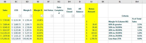
For example, if the job achieved a margin of 50.64% on a sale of $2,879.58, then the employee would be paid 2% of the sale (or $57.59) base on the below criteria:

Margin % (Column BE)	% of Total Sales
60% & greater	2.5%​
50% to 59.99%	2.0%​
40% to 49.99%	1.5%​
30% to 39.99%	1.0%​
25% to 29.99%	0.5%​
Less than 25%	0.0%​

I'd like for the spreadsheet to be plug & play where I can dump data into it and it auto determines the % bonus without me having to manually complete this.

I can provide a sample of the spreadsheet if required.

Thank you,

 

[offthelip]

try this:

=IF(BE5>60%,2.5,IF(BE5<25%,0,0.5*INT((BE5-0.1)*10)))

 

[JenMcG]

try this:

=IF(BE5>60%,2.5,IF(BE5<25%,0,0.5*INT((BE5-0.1)*10)))

Hello,

Thank you. I have inserted this as a helper column to use as the multiplier. The issue is the number is not returned as a percentage and when converted to a percentage the percentages become 50%, 100%, 150%, 200% & 250%. However, I need them to be at .50%, 1.5%, 2%, & 2.5%.

How can I correct this?

 

[offthelip]

just multiply by 0.01:

=0.01*IF(E5>60%,2.5,IF(E5<25%,0,0.5*INT((E5-0.1)*10)))

 

[JenMcG]

just multiply by 0.01:

=0.01*IF(E5>60%,2.5,IF(E5<25%,0,0.5*INT((E5-0.1)*10)))

Thank you!

 

[JenMcG]

just multiply by 0.01:

=0.01*IF(E5>60%,2.5,IF(E5<25%,0,0.5*INT((E5-0.1)*10)))

Hi Again,

While this formula worked for this specific percentages, I don't know that I fully understand it if I want to alter the ranges and percentages. Are you able to break it down for me so I can alter the ranges and percentages easily?

Thank you,

 

[offthelip]

With the ranges and the percentages that you specified I identified that they were both linear once you were in the range 20% to 60% given that less that 25% was zero.
So the calculation takes input percentage 20%, 30 % 40% plus some small value, subtracts 10% (-0.1) then divides it by 10 and then takes the integer value of this, so 28% minus 10% equals 18% divide by 10 gives 1.8 n then take the interger which gives you 1 multiply by 0.5 gives you the 0.5% you want for the bonus. another example 34% minus 10%= 24% , divided by 10 give 2.4% take integer gives 2 times 0.5 gives 1
If you want to change the values to something that is not linear then this will not work,

 

[JenMcG]

With the ranges and the percentages that you specified I identified that they were both linear once you were in the range 20% to 60% given that less that 25% was zero.
So the calculation takes input percentage 20%, 30 % 40% plus some small value, subtracts 10% (-0.1) then divides it by 10 and then takes the integer value of this, so 28% minus 10% equals 18% divide by 10 gives 1.8 n then take the interger which gives you 1 multiply by 0.5 gives you the 0.5% you want for the bonus. another example 34% minus 10%= 24% , divided by 10 give 2.4% take integer gives 2 times 0.5 gives 1
If you want to change the values to something that is not linear then this will not work,

Thank you.

Is there another option if we'd like to explore non linear values? For example: could we setup a box were we can alter the ranges (of percentages) and the multiple in a separate part of the sheet (outside of the chart) and can a formula pull from that?

Or a more complex formula where we can alter the ranges and multiples within it?

Thanks,

 

[offthelip]

You could do it quite easily using a vlookup on another sheet, If you put the numbers 1 to 100 in rows 1 to 100 in column A on a new worksheet and rename it "Bonus" Then for each row put in the percentage bonus you want in column B for that percentage e.g. for your original , zero for rows 1 to 24 , 0.5 for rows 25 to 29, then 1 for 30 to 39, etc , the this formula will work:

=VLOOKUP(INT(100*E4),Bonus!A$1:B$60,2)

 

[JenMcG]

You could do it quite easily using a vlookup on another sheet, If you put the numbers 1 to 100 in rows 1 to 100 in column A on a new worksheet and rename it "Bonus" Then for each row put in the percentage bonus you want in column B for that percentage e.g. for your original , zero for rows 1 to 24 , 0.5 for rows 25 to 29, then 1 for 30 to 39, etc , the this formula will work:

=VLOOKUP(INT(100*E4),Bonus!A$1:B$60,2)

Perfect! This works- thx again