Calculate cumulative commissions with tiers

[vdam]

Commissions with thresholds
I have to calculate commission taking into account statistical amount for cycle. Please help find formula in excel?

• Amount 1: 1000.00 EUR,
• Amount 2: 1500.00 EUR.

There are rules set up defining that we should apply:

• A1 - for amount <= 500.00 (0%)
• B89 - for amount from 500.01 to 700.00 (2%)
• B66 - for amount >700.00 (1%, min 5.00eur)

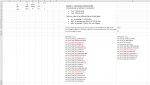
For Amount 1 following commissions was calculated: A1 on 500 (0.00 EUR), B89 on 200 (4.00 EUR) , B66 on 300 (5.00 EUR).

For Amount 2 B66 on 2500 was calculated, because of accumulated amount. Amount already was >700, so B66 was used.

 

[CA_Punit]

I have a doubt

Please reply for Amount 1 =800
Amount 2 =100

What should be the Result.

As Amount 800 Exceed Rs 700 so It should be 0+4+5
As amount already exceed Rs 700 so on 100 should it be 5 or (combine 100 from Amount 1 and Amount 2 =200 and 1% on 200 is 2 subject to min of 5 ie Total considering both should be 5)

 

[vdam]

I have a doubt

Please reply for Amount 1 =800
Amount 2 =100

What should be the Result.

As Amount 800 Exceed Rs 700 so It should be 0+4+5
As amount already exceed Rs 700 so on 100 should it be 5 or (combine 100 from Amount 1 and Amount 2 =200 and 1% on 200 is 2 subject to min of 5 ie Total considering both should be 5)

For Amount 1 (800) would be 0+4+5, For amount 2 (100) would be 5

 

[vdam]

In picture task more clear

 

[CA_Punit]

After going through the probelm it is easy to find the commission if the first value falls in the Third category i.e. above 700. However if you see a scenerio of say 550 in Amount 1 and 200 in Amount 2. Which complicates the issue. I have to take 150 @ .02 and have to check the remaining 50*.01 subject to minimum of 5.

I could not come up with a solution for the second Amount


If i may request @Eric W if he could help us solve this.

 

[CA_Punit]

Desktop11.xlsx
	B	C	D	E	F
1
2		Cumulative	Rate	Incremental Rate
3		0	0	0
4		500	0	0
5		700	0.02	0.02
6		100001	0.01	0.03
7
8
9
10
11
12
13
14
15		450	0
16		200
17
Sheet1

Cell Formulas
Range	Formula
E3:E6	E3	=SUM($D$2:D3)
D15	D15	=SUM(IFERROR(IF((IF(((C15-C3:C6)*(C15>=C3:C6))<=((C4:C7-C3:C6)*(C15>=C3:C6)),((C15-C3:C6)*(C15>=C3:C6)),((C4:C7-C3:C6)*(C15>=C3:C6)))*(E4:E7-E3:E6))>=IF(C15>700,{0;0;5},{0;0;0}),(IF(((C15-C3:C6)*(C15>=C3:C6))<=((C4:C7-C3:C6)*(C15>=C3:C6)),((C15-C3:C6)*(C15>=C3:C6)),((C4:C7-C3:C6)*(C15>=C3:C6)))*(E4:E7-E3:E6)),{0;0;5}),0))

This is what i tried

 

[Dave Patton]

For total commission, try either of the following

T202009b.xlsm
	A	B	C	D
1
2		Cumulative	Rate	Rate Diff
3		0	0	0
4		500	0.02	0.02
5		700	0.01	-0.01
6
7		750	5.00	5.00
8		5000	47.00	47.00
1f

Cell Formulas
Range	Formula
D3:D5	D3	=C3-N(C2)
C7:C8	C7	=MAX(5,SUMPRODUCT(--(B7>$B$3:$B$5),B7-$B$3:$B$5,$D$3:$D$5))
D7:D8	D7	=MAX(5,(B7>$B$4)*MIN($B$5-$B$4,B7-$B$4)*$C$4+(B7>$B$5)*(B7-$B$5)*$C$5)

 

[CA_Punit]

For total commission, try either of the following

T202009b.xlsm
	A	B	C	D
1
2		Cumulative	Rate	Rate Diff
3		0	0	0
4		500	0.02	0.02
5		700	0.01	-0.01
6
7		750	5.00	5.00
8		5000	47.00	47.00
1f

Cell Formulas
Range	Formula
D3:D5	D3	=C3-N(C2)
C7:C8	C7	=MAX(5,SUMPRODUCT(--(B7>$B$3:$B$5),B7-$B$3:$B$5,$D$3:$D$5))
D7:D8	D7	=MAX(5,(B7>$B$4)*MIN($B$5-$B$4,B7-$B$4)*$C$4+(B7>$B$5)*(B7-$B$5)*$C$5)

Hi @Dave Patton

Your Formula doesn't meet the his requirement.
If i change the Amount 1 to 250, it still shows 5.

 

[Dave Patton]

T202009b.xlsm
	A	B	C	D
1
2		Cumulative	Rate	Rate Diff
3		0	0	0
4		500	0.02	0.02
5		700	0.01	-0.01
6
7		250	0.00	0.00
8		5000	47.00	47.00
1f

Cell Formulas
Range	Formula
D3:D5	D3	=C3-N(C2)
C7	C7	=MAX((B7>$B$5)*5,SUMPRODUCT(--(B7>$B$3:$B$5),B7-$B$3:$B$5,$D$3:$D$5))
D7:D8	D7	=MAX((B7>$B$5)*5,(B7>$B$4)*MIN($B$5-$B$4,B7-$B$4)*$C$4+(B7>$B$5)*(B7-$B$5)*$C$5)
C8	C8	=MAX(5,SUMPRODUCT(--(B8>$B$3:$B$5),B8-$B$3:$B$5,$D$3:$D$5))

 

[CA_Punit]

T202009b.xlsm
	A	B	C	D
1
2		Cumulative	Rate	Rate Diff
3		0	0	0
4		500	0.02	0.02
5		700	0.01	-0.01
6
7		250	0.00	0.00
8		5000	47.00	47.00
1f

Cell Formulas
Range	Formula
D3:D5	D3	=C3-N(C2)
C7	C7	=MAX((B7>$B$5)*5,SUMPRODUCT(--(B7>$B$3:$B$5),B7-$B$3:$B$5,$D$3:$D$5))
D7:D8	D7	=MAX((B7>$B$5)*5,(B7>$B$4)*MIN($B$5-$B$4,B7-$B$4)*$C$4+(B7>$B$5)*(B7-$B$5)*$C$5)
C8	C8	=MAX(5,SUMPRODUCT(--(B8>$B$3:$B$5),B8-$B$3:$B$5,$D$3:$D$5))

Hi @Dave Patton

If it is 701 your formula results in 5, whereas it should return 4+5=9
700-500=200*.02=4
701-700=1*.01 Min 5 = 5

Also there is second Amount also which is dependent on the First. If the First falls in 500-700 , then we have to first complete the 500-700 range from the second amount and the remaining amount of Amount 2 should be used with more than 700 criteria