Dear Friends,
I have a Raw Data Like this:
From this data I am able to get result in this format for a single fruit:
Guava is a Drop Down List here, Stock Date & Qty i.e. 200 is manually entered, rest results i.e. from SUPPLIER to Value are formula driven:
For SUPPLIER : =IF($L3="","",INDEX(B$3:B$9,MATCH($L3,$D$3:$D$9,0)))
INV NO : =IF($L3="","",INDEX(C$3:C$9,MATCH($L3,$D$3:$D$9,0)))
DATE : =IFERROR(AGGREGATE(15,6,D$3:D$9/($A$3:$A$9=$H$3)/(D$3:D$9<=$I$1),ROWS($1:1)),"")
RATE: =IF($L3="","",INDEX(F$3:F$9,MATCH($L3,$D$3:$D$9,0)))
PURCHASE : =IF($L3="","",INDEX(E$3:E$9,MATCH($L3,$D$3:$D$9,0)))
SELL : =IF($L3="","",MIN($N3,MAX(0,SUM($N$3:$N$8)-I$3-SUM(O$2:O2))))
STOCK (BALANCE) =IF($L3="","",$N3-$O3)
VALUE : =IFERROR(P3*M3,"")
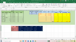
Now my problem is till this I am able to give stock valuation for a single fruit only but my modified & latest format is changed & now need result in the form mentioned below:
FRUIT & STOCK these two columns are already available, rest all I need formulas & desired results would be in the same form, please note in case if I take reference from my previous formula driven cells, then if Stock (Balance) becomes 0, that would be ignored. for better understanding I have uploaded an image of my file. From F14 to J16 is my desired result. Yellow cells & Red fonts are my present formula driven results.
Please help, please note that in original sheet there are about more than 10000 data of fruits & result for Suppliers, dates etc may come more than 10 nos.
Regards
RAMU
I have a Raw Data Like this:
| PURCHASE | |||||
| FRUIT | SUPPLIER | INV NO | DATE | QTY | RATE |
| GUAVA | GK TRADER | 10 | 10-04-2021 | 96 | 8 |
| APPLE | SM | 102 | 09-04-2021 | 50 | 12 |
| BANANA | SM | 134 | 12-05-2021 | 144 | 3 |
| APPLE | GK TRADER | 15 | 19-05-2021 | 252 | 10 |
| BANANA | SOM | 35/58 | 05-05-2021 | 180 | 3.25 |
| APPLE | SOM | 35/59 | 17-05-2021 | 192 | 11.5 |
| GUAVA | SM | 149 | 22-05-2021 | 120 | 7.3 |
From this data I am able to get result in this format for a single fruit:
| STOCK DATE : | 13-06-2021 | SUPPLIER | INV NO | DATE | RATE | ||||
| Purchase | Sell | Stock (Balance) | Value | ||||||
| GUAVA | 200 | GK TRADER | 10 | 10-04-2021 | 8 | 96 | 16 | 80 | 640 |
| SM | 149 | 22-05-2021 | 7.3 | 120 | 0 | 120 | 876 | ||
| | Total | 216 | 16 | 200 | 1516 |
Guava is a Drop Down List here, Stock Date & Qty i.e. 200 is manually entered, rest results i.e. from SUPPLIER to Value are formula driven:
For SUPPLIER : =IF($L3="","",INDEX(B$3:B$9,MATCH($L3,$D$3:$D$9,0)))
INV NO : =IF($L3="","",INDEX(C$3:C$9,MATCH($L3,$D$3:$D$9,0)))
DATE : =IFERROR(AGGREGATE(15,6,D$3:D$9/($A$3:$A$9=$H$3)/(D$3:D$9<=$I$1),ROWS($1:1)),"")
RATE: =IF($L3="","",INDEX(F$3:F$9,MATCH($L3,$D$3:$D$9,0)))
PURCHASE : =IF($L3="","",INDEX(E$3:E$9,MATCH($L3,$D$3:$D$9,0)))
SELL : =IF($L3="","",MIN($N3,MAX(0,SUM($N$3:$N$8)-I$3-SUM(O$2:O2))))
STOCK (BALANCE) =IF($L3="","",$N3-$O3)
VALUE : =IFERROR(P3*M3,"")
Now my problem is till this I am able to give stock valuation for a single fruit only but my modified & latest format is changed & now need result in the form mentioned below:
| FRUIT | STOCK | SUPPLIERS | DATES | INV NOS | QTY | VALUE |
| APPLE | 300 | GK TRADER, SOM | 19-05-21, 17-05-21 | 15, 35/59 | 252, 48 | 3072 |
| BANANA | 300 | SM, SOM | 12-05-21, 05-05-21 | 134, 35/58 | 144, 156 | 939 |
| GUAVA | 200 | SM, GK TRADER | 22-05-21, 10-04-21 | 149, 10 | 120, 80 | 1516 |
FRUIT & STOCK these two columns are already available, rest all I need formulas & desired results would be in the same form, please note in case if I take reference from my previous formula driven cells, then if Stock (Balance) becomes 0, that would be ignored. for better understanding I have uploaded an image of my file. From F14 to J16 is my desired result. Yellow cells & Red fonts are my present formula driven results.
Please help, please note that in original sheet there are about more than 10000 data of fruits & result for Suppliers, dates etc may come more than 10 nos.
Regards
RAMU