Call Center Stat Help: Ranking Full-Time and Part-Time Employees

[life_in_picture_format]

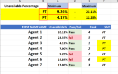
Hi, I have a multi page spreadsheet that is calculating the averages of specifc call center metrics and provides us with an overall grade/ranking for thhe employees. One metrics is Average Unavailable Percentage. Basically if 100% = the total time our Agent was logged on to the sysetem we measure how much if that 100 % was spent in a non working mode. That is what I am measuring here.
In my attached image I am showing what I want the calculation to do.

The thing I'm stumped by is how to rank ALL employees when there is a mix of Full-Time(FT) and Part-Time(PT) employees, each have a different range of allowable unavailable time a month.

%-FT have a range of 9.26% - 21.11 % while PT has a range of 4.17%-11.25%. How do you calculate such to trigger a Pass or Fail in column D AND rank them based upon whoever is closest to the MINIMUM with out going below Minimum. If you notice anything below minimum is worse than being over.

Please assist, thank you

 

[Eric W]

Welcome to the MrExcel forum!

Try:

Book1
	A	B	C	D	E	F
1	Unavailable Percentage		Minimum		Maximum
2		FT	9.26%		21.11%
3		PT	4.17%		11.25%
4
5	First Name	Last Name	Unavailable %	Pass/Fail	Rank	Shift
6	Agent	1	20.13%	Pass	4	FT
7	Agent	2	22.37%	fail	7	FT
8	Agent	3	4.19%	Pass	1	PT
9	Agent	4	7.00%	Pass	2	PT
10	Agent	5	9.20%	fail	5	FT
11	Agent	6	14.84%	fail	6	PT
12	Agent	7	17.00%	Pass	3	FT
13
Sheet8

Cell Formulas
Range	Formula
D6:D12	D6	=IF(AND(C6>=VLOOKUP(F6,$B$2:$E$3,2,0),C6<=VLOOKUP(F6,$B$2:$E$3,4,0)),"Pass","fail")
E6:E12	E6	=SUMPRODUCT(--($C$6:$C$12-VLOOKUP($F$6:$F$12,$B$2:$E$3,2,0)+($D$6:$D$12="fail")*100<=C6-VLOOKUP(F6,$B$2:$E$3,2,0)+(D6="fail")*100))

Cells with Conditional Formatting
Cell	Condition		Cell Format	Stop If True
D6:D12	Cell Value	contains "fail"	text	NO

 

[life_in_picture_format]

Hello sir, thank you for your assistance and taking the time to help. The only thing missing is ranking those who are below the minimum as worse than those under. Agent 5 should be last place because they did not take enough break time which is bad because they are working against state employment laws and the company can get in trouble. Is there a way to rank those as a negative?

I do appreciate you!

 

[life_in_picture_format]

Hello sir, thank you for your assistance and taking the time to help. The only thing missing is ranking those who are below the minimum as worse than those under. Agent 5 should be last place because they did not take enough break time which is bad because they are working against state employment laws and the company can get in trouble. Is there a way to rank those as a negative?

I do appreciate you!

worse than those who are OVER not under, my apologies

 

[life_in_picture_format]

Welcome to the MrExcel forum!

Try:

Book1
	A	B	C	D	E	F
1	Unavailable Percentage		Minimum		Maximum
2		FT	9.26%		21.11%
3		PT	4.17%		11.25%
4
5	First Name	Last Name	Unavailable %	Pass/Fail	Rank	Shift
6	Agent	1	20.13%	Pass	4	FT
7	Agent	2	22.37%	fail	7	FT
8	Agent	3	4.19%	Pass	1	PT
9	Agent	4	7.00%	Pass	2	PT
10	Agent	5	9.20%	fail	5	FT
11	Agent	6	14.84%	fail	6	PT
12	Agent	7	17.00%	Pass	3	FT
13
Sheet8

Cell Formulas
Range	Formula
D6:D12	D6	=IF(AND(C6>=VLOOKUP(F6,$B$2:$E$3,2,0),C6<=VLOOKUP(F6,$B$2:$E$3,4,0)),"Pass","fail")
E6:E12	E6	=SUMPRODUCT(--($C$6:$C$12-VLOOKUP($F$6:$F$12,$B$2:$E$3,2,0)+($D$6:$D$12="fail")*100<=C6-VLOOKUP(F6,$B$2:$E$3,2,0)+(D6="fail")*100))

Cells with Conditional Formatting
Cell	Condition		Cell Format	Stop If True
D6:D12	Cell Value	contains "fail"	text	NO

Not sure if you will see my message above since I didn't select "reply" so here it is lol

 

[Eric W]

I was afraid you'd want that. Try:

Book1
	A	B	C	D	E	F	G
1	Unavailable Percentage		Minimum		Maximum
2		FT	9.26%	0	21.11%
3		PT	4.17%	0	11.25%
4
5	First Name	Last Name	Unavailable %	Pass/Fail	Rank	Shift
6	Agent	1	20.13%	Pass	4	FT	0.1087
7	Agent	2	22.37%	fail	5	FT	100.0126
8	Agent	3	4.19%	Pass	1	PT	0.0002
9	Agent	4	7.00%	Pass	2	PT	0.0283
10	Agent	5	9.20%	fail	7	FT	200.0006
11	Agent	6	14.84%	fail	6	PT	100.0359
12	Agent	7	17.00%	Pass	3	FT	0.0774
13
Sheet8

Cell Formulas
Range	Formula
D6:D12	D6	=IF(PRODUCT(C6-VLOOKUP(F6,$B$2:$E$3,{2,4},0))>0,"fail","Pass")
E6:E12	E6	=RANK(G6,$G$6:$G$12,1)
G6:G12	G6	=IF(C6<VLOOKUP(F6,$B$2:$E$3,2,0),200+VLOOKUP(F6,$B$2:$E$3,2,0)-C6,IF(D6="fail",C6-VLOOKUP(F6,$B$2:$E$3,4,0)+100,C6-VLOOKUP(F6,$B$2:$E$3,2,0)))

Cells with Conditional Formatting
Cell	Condition		Cell Format	Stop If True
D6:D12	Cell Value	contains "fail"	text	NO

The size of the E formula was getting out of hand, so I made a helper column in G. You can hide that column if you want. Then the E formula is pretty simple. I found a shorter formula for the D column (but it's a bit more arcane, so you may want to stick with the first one).

 

[life_in_picture_format]

I was afraid you'd want that. Try:

Book1
	A	B	C	D	E	F	G
1	Unavailable Percentage		Minimum		Maximum
2		FT	9.26%	0	21.11%
3		PT	4.17%	0	11.25%
4
5	First Name	Last Name	Unavailable %	Pass/Fail	Rank	Shift
6	Agent	1	20.13%	Pass	4	FT	0.1087
7	Agent	2	22.37%	fail	5	FT	100.0126
8	Agent	3	4.19%	Pass	1	PT	0.0002
9	Agent	4	7.00%	Pass	2	PT	0.0283
10	Agent	5	9.20%	fail	7	FT	200.0006
11	Agent	6	14.84%	fail	6	PT	100.0359
12	Agent	7	17.00%	Pass	3	FT	0.0774
13
Sheet8

Cell Formulas
Range	Formula
D6:D12	D6	=IF(PRODUCT(C6-VLOOKUP(F6,$B$2:$E$3,{2,4},0))>0,"fail","Pass")
E6:E12	E6	=RANK(G6,$G$6:$G$12,1)
G6:G12	G6	=IF(C6<VLOOKUP(F6,$B$2:$E$3,2,0),200+VLOOKUP(F6,$B$2:$E$3,2,0)-C6,IF(D6="fail",C6-VLOOKUP(F6,$B$2:$E$3,4,0)+100,C6-VLOOKUP(F6,$B$2:$E$3,2,0)))

Cells with Conditional Formatting
Cell	Condition		Cell Format	Stop If True
D6:D12	Cell Value	contains "fail"	text	NO

The size of the E formula was getting out of hand, so I made a helper column in G. You can hide that column if you want. Then the E formula is pretty simple. I found a shorter formula for the D column (but it's a bit more arcane, so you may want to stick with the first one).

You are AMAZING!!!! <3

 

[Eric W]

Glad I could help! ?