Check result of formula and change to a list value

ollyhughes1982

Well-known Member
Joined
Nov 27, 2018
Messages
677
Office Version
  1. 365
Platform
  1. MacOS
Hi,

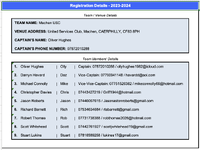
I have a pool league results card that I complete each week, for my team’s personal use and records. This is fine, but in this I use our ‘short’ names, rather than our official full names. See image below:

Screenshot 2023-11-21 at 20.50.31.jpg


However, when I post the result card to the league, I’d like it show our full names. Is there a way in Excel that I could have a version where the formulas in each cell checks the result and then a further part of the formula chooses the correct full name from a lookup list? I’m aware that this is a little odd, as it is a formula that will look at the result within the same formula to then do a lookup and change the value.

e.g. Olly should change to Oliver Hughes, Stuart to Stuart Bloggs, Mike to Michael Jones and so on...

I always record the full names of opposition anyway, so these won't need changing.

File is here: Pool Team (Division 1, 2023-2024) WORKING.xlsx

Thanks in advance!

Olly.
 

Excel Facts

Which lookup functions find a value equal or greater than the lookup value?
MATCH uses -1 to find larger value (lookup table must be sorted ZA). XLOOKUP uses 1 to find values greater and does not need to be sorted.
In this example, each player has a Player ID

Cell B1 is the choice to show short or full names which changes all the results throughout the workbook. Range A4:B4 is the working example. Range I1:K4 is the player table

Book1
ABCDEFGHIJK
1FullPlayer IDShort NameFull Name
21001OllyOlliver Hughes
31002StuartStuart Bloggs
41002Stuart Bloggs1003MikeMichael Jones
5
6
Sheet2
Cell Formulas
RangeFormula
B4B4=VLOOKUP(A4,PlayerTbl,IF(NameSelection="Short",2,3),FALSE)
Named Ranges
NameRefers ToCells
NameSelection=Sheet2!$B$1B4
PlayerTbl=Sheet2!$I$2:$K$4B4
Cells with Data Validation
CellAllowCriteria
B1ListShort,Full
 
Upvote 0
In this example, each player has a Player ID

Cell B1 is the choice to show short or full names which changes all the results throughout the workbook. Range A4:B4 is the working example. Range I1:K4 is the player table

Book1
ABCDEFGHIJK
1FullPlayer IDShort NameFull Name
21001OllyOlliver Hughes
31002StuartStuart Bloggs
41002Stuart Bloggs1003MikeMichael Jones
5
6
Sheet2
Cell Formulas
RangeFormula
B4B4=VLOOKUP(A4,PlayerTbl,IF(NameSelection="Short",2,3),FALSE)
Named Ranges
NameRefers ToCells
NameSelection=Sheet2!$B$1B4
PlayerTbl=Sheet2!$I$2:$K$4B4
Cells with Data Validation
CellAllowCriteria
B1ListShort,Full
I'll give this a try. Thanks
 
Upvote 0
I'm not sure if this is what I'm after. i want the formula in G14, G16, G18 etc. to be able to look at what the result of the formula is and then lookup from the 'Registration Details - 23-24' worksheet what the full name should be and display that.
 
Upvote 0
i want the formula in G14, G16, G18 etc. to be able to look at what the result of the formula is and then lookup from the 'Registration Details - 23-24' worksheet what the full name should be
G14 contains "Olly". I don't see anything on 'Registration Details - 23-24' that logically links the name "Olly" to any of the 9 names listed on that worksheet. Even less for "Daz" in G22.
 
Upvote 0
G14 contains "Olly". I don't see anything on 'Registration Details - 23-24' that logically links the name "Olly" to any of the 9 names listed on that worksheet. Even less for "Daz" in G22.
Apologies, I thought I had uploaded a new version with this mapped in. I have now added this.

You can now find this updated file at the same link. I think I have now solved this with the formula you will be able to see in G14 and AT14, shown below:

G14:
Excel Formula:
=XLOOKUP(IF('Match Card # 1'!$A$3="Home",'Match Card # 1'!B4,'Match Card # 1'!H4),'Registration Details - 23-24'!$AD$10:$AD$18,'Registration Details - 23-24'!$J$10:$J$18,IF('Match Card # 1'!$A$3="Home",'Match Card # 1'!B4,'Match Card # 1'!H4))

AT14:
Excel Formula:
=XLOOKUP(IF('Match Card # 1'!$A$3="Away",'Match Card # 1'!B4,'Match Card # 1'!H4),'Registration Details - 23-24'!AD10:AD18,'Registration Details - 23-24'!J10:J18,IF('Match Card # 1'!$A$3="Away",'Match Card # 1'!B4,'Match Card # 1'!H4))

Thanks.
 

Attachments

  • Screenshot 2023-11-22 at 08.16.29.png
    Screenshot 2023-11-22 at 08.16.29.png
    184.1 KB · Views: 2
Upvote 0
Apologies, I thought I had uploaded a new version with this mapped in. I have now added this.

You can now find this updated file at the same link. I think I have now solved this ..
In that case could you use these considerably shorter formulas?
G14:
Excel Formula:
=LET(n,INDEX('Match Card # 1'!B4:H4,1+6*('Match Card # 1'!$A$3="Away")),lur,'Registration Details - 23-24'!J10:AD18,XLOOKUP(n,TAKE(lur,,-1),TAKE(lur,,1),n))
AT14:
Excel Formula:
=LET(n,INDEX('Match Card # 1'!B4:H4,1+6*('Match Card # 1'!$A$3="Home")),lur,'Registration Details - 23-24'!J10:AD18,XLOOKUP(n,TAKE(lur,,-1),TAKE(lur,,1),n))
 
Upvote 1
Solution
In that case could you use these considerably shorter formulas?
G14:
Excel Formula:
=LET(n,INDEX('Match Card # 1'!B4:H4,1+6*('Match Card # 1'!$A$3="Away")),lur,'Registration Details - 23-24'!J10:AD18,XLOOKUP(n,TAKE(lur,,-1),TAKE(lur,,1),n))
AT14:
Excel Formula:
=LET(n,INDEX('Match Card # 1'!B4:H4,1+6*('Match Card # 1'!$A$3="Home")),lur,'Registration Details - 23-24'!J10:AD18,XLOOKUP(n,TAKE(lur,,-1),TAKE(lur,,1),n))
Thanks 👍🏻
 
Upvote 0

Forum statistics

Threads
1,215,069
Messages
6,122,959
Members
449,096
Latest member
Anshu121

We've detected that you are using an adblocker.

We have a great community of people providing Excel help here, but the hosting costs are enormous. You can help keep this site running by allowing ads on MrExcel.com.
Allow Ads at MrExcel

Which adblocker are you using?

Disable AdBlock

Follow these easy steps to disable AdBlock

1)Click on the icon in the browser’s toolbar.
2)Click on the icon in the browser’s toolbar.
2)Click on the "Pause on this site" option.
Go back

Disable AdBlock Plus

Follow these easy steps to disable AdBlock Plus

1)Click on the icon in the browser’s toolbar.
2)Click on the toggle to disable it for "mrexcel.com".
Go back

Disable uBlock Origin

Follow these easy steps to disable uBlock Origin

1)Click on the icon in the browser’s toolbar.
2)Click on the "Power" button.
3)Click on the "Refresh" button.
Go back

Disable uBlock

Follow these easy steps to disable uBlock

1)Click on the icon in the browser’s toolbar.
2)Click on the "Power" button.
3)Click on the "Refresh" button.
Go back
Back
Top