Cleanup Credit Card Merchant Names Using VBA

austinb

New Member
Joined
Feb 24, 2021
Messages
19
Office Version
  1. 365
  2. 2013
Platform
  1. Windows
Hello all,

I'm basically looking to create a macro that will search a column of cells for text from a list located on another tab and if found, replaces the text in the original cell with the text from the cell in the other tab.

For example,in Sheet1, B2 = 7-ELEVEN 38587 00073PITTSBURGH PA & B3 = 7-ELEVEN 38671 00073COPPELL TX

I would like the macro to search data found in Sheet2 for "7-ELEVEN" (not case sensitive) and replace both cells B2 & B3 in Sheet1 with just "7-Eleven".

This is somewhat of a continuation of a posted question that hasn't been updated since August of 2019 (Bank Transaction Description/Merchant Cleanup & Auto Categorize (like Mint)).

I am a VBA newbie and any help would be greatly appreciated. Thank you

-Austin
 

Excel Facts

Why are there 1,048,576 rows in Excel?
The Excel team increased the size of the grid in 2007. There are 2^20 rows and 2^14 columns for a total of 17 billion cells.
Sample worksheets make this easier to help. Use XL2BB and provide some sample data and then show us a mocked up solution for the sample data.
 
Upvote 0
Hello can you please help understanding the query better ?

Suppose in sheet2 B2 there is "7-Eleven" and in C2 is " austin" , so in sheet1 what do you want in the cells B2 &B3
1. 7-Eleven

Or
2. austin

Regards
Neha
 
Upvote 0
Thank you both for your time looking into my questions. Here is some sample data (hopefully this works).

Data in Sheet 1
activity.csv
ABC
1DateDescriptionAmount
21/29/20217-ELEVEN 38587 00073PITTSBURGH PA5.67
32/8/20217-ELEVEN 38671 00073COPPELL TX49.50
42/14/2021Abbey Resort-455.80
52/20/2021ADOBE CREATIVE CLOUDSAN JOSE CA55.90
62/4/2021ADOBE PHOTOGPHY PLANSAN JOSE CA10.54
72/3/2021ADOBE PS CREATIVE CLSAN JOSE CA22.14
82/20/2021Adobe Systems Incorporated15.81
92/19/2021AMAZON KIDS+*DU9FX5D888-802-3080 WA6.99
102/3/2021Amazon Web Services1647.36
112/19/2021Amazon.com248.24
122/20/2021AMAZON.COM*G03ZN92W3AMZN.COM/BILL WA80.80
132/3/2021AMAZON.COM*GX93V14H3AMZN.COM/BILL WA1486.49
142/8/2021AMAZON.COM*PD7207QO3AMZN.COM/BILL WA46.41
152/16/2021American Airlines255.81
162/6/2021AMERICAN AIRLINES 800-433-7300 TX750.40
Data Entry


Data in Sheet 2
activity.csv
B
1Number
27-Eleven
3Adobe Systems Incorporated
4Amazon Web Services
5Amazon.com
6American Airlines
CoA, Vendors, Dept, Classes
 
Upvote 0
And here is how I would like the Data in Sheet 1 to appear after the macro

activity.csv
ABC
1DateDescriptionAmount
21/29/20217-Eleven5.67
32/8/20217-Eleven49.50
42/14/2021Abbey Resort-455.80
52/20/2021Adobe Systems Incorporated55.90
62/4/2021Adobe Systems Incorporated10.54
72/3/2021Adobe Systems Incorporated22.14
82/20/2021Adobe Systems Incorporated15.81
92/19/2021AMAZON KIDS+*DU9FX5D888-802-3080 WA6.99
102/3/2021Amazon Web Services1647.36
112/19/2021Amazon.com248.24
122/20/2021Amazon.com80.80
132/3/2021Amazon.com1486.49
142/8/2021Amazon.com46.41
152/16/2021American Airlines255.81
162/6/2021American Airlines750.40
Data Entry
 
Upvote 0
Look at this tutorial on doing a fuzzy match in Power Query

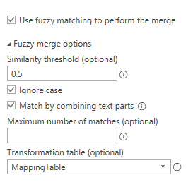
Thank you for this. I had downloaded the Fuzzy Lookup add-in long ago but never really learned how to use it. I have now downloaded the Power Query Add-In and went through the steps but I am not seeing the "Use fuzzy matching to perform the merge" option when combining my queries.

This is what I get:

1614270014769.png
 
Upvote 0
OK, I think I've got it working with the Fuzzy Lookup add-in. Thank you very much for pointing me in the right direction Alan. I really appreciate it!
 
Upvote 0
Hello I am also providing you with the macro, I hope it works for you, Please let me know if this solves your query

VBA Code:
Sub mycode()
Dim lastrowsh1 As Integer
Dim lastrowsh2 As Integer

Dim cell1 As Range
Dim cell2 As Range

lastrowsh1 = Sheets(1).Range("a2").End(xlDown).Row
lastrowsh2 = Sheets(2).Range("a2").End(xlDown).Row

    For Each cell1 In Sheets(1).Range("b2:b" & lastrowsh1)
        For Each cell2 In Sheets(2).Range("a2:a" & lastrowsh2)
            If InStr(1, UCase(cell1.Value), UCase(cell2.Value), 1) <> 0 Then
                cell1.Value = cell2.Value
                Exit For
            End If
        Next cell2
    Next cell1
End Sub
Hi Neha,

Thank you for your time however I could not get this to work for me. It doesn't appear to be doing anything when I run it.
 
Upvote 0

Forum statistics

Threads
1,215,440
Messages
6,124,882
Members
449,193
Latest member
PurplePlop

We've detected that you are using an adblocker.

We have a great community of people providing Excel help here, but the hosting costs are enormous. You can help keep this site running by allowing ads on MrExcel.com.
Allow Ads at MrExcel

Which adblocker are you using?

Disable AdBlock

Follow these easy steps to disable AdBlock

1)Click on the icon in the browser’s toolbar.
2)Click on the icon in the browser’s toolbar.
2)Click on the "Pause on this site" option.
Go back

Disable AdBlock Plus

Follow these easy steps to disable AdBlock Plus

1)Click on the icon in the browser’s toolbar.
2)Click on the toggle to disable it for "mrexcel.com".
Go back

Disable uBlock Origin

Follow these easy steps to disable uBlock Origin

1)Click on the icon in the browser’s toolbar.
2)Click on the "Power" button.
3)Click on the "Refresh" button.
Go back

Disable uBlock

Follow these easy steps to disable uBlock

1)Click on the icon in the browser’s toolbar.
2)Click on the "Power" button.
3)Click on the "Refresh" button.
Go back
Back
Top