Combine 3 different index-match functions but referencing 1 specific helper cell

[derman0524]

Hi there, I've been struggling to get the index-match function to work properly with more than 1 index match.

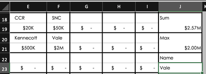
Basically, below are 3 different 'rows', where each column is 1 week across a full month. In the Name tab at the bottom right, I want to output the correct text above the MAX value in this entire array. I'm able to do single index match but I can't seem to correctly add multiple index arrays when they're on different row numbers.

Currently: =INDEX(E20:I20,MATCH($J$21,E21:I21,0)) which outputs Vale, as it correctly found the matched the max value with the index row array just above it, but I can't seem to figure out how to make add multiple rows to the index array if they're on different rows.

My other thinking is to have some sort of index nested function with some if statements to output the MAX value and attach the Name to that max value across the entire array.

Let me know. Thanks!

 

[Cubist]

Maybe this.

Book1
	A	B	C	D	E	F
1	CCr	SNC
2	$ 20,000	$ 50,000			Sum	$ 13,570,000
3	Kennecott	Vale		Kevin	Max	$ 8,000,000
4	$ 500,000	$ 2,000,000		$ 3,000,000	Name	Valerie
5			Valerie
6	$ -	$ -	$ 8,000,000
Sheet3

Cell Formulas
Range	Formula
F2	F2	=SUM(A1:D6)
F3	F3	=MAX(A1:D6)
F4	F4	=LET(w,WRAPROWS(TOCOL(A1:D6,,TRUE),2),FILTER(CHOOSECOLS(w,1),CHOOSECOLS(w,2)=MAX(w)))

 

[derman0524]

Maybe this.

Book1
	A	B	C	D	E	F
1	CCr	SNC
2	$ 20,000	$ 50,000			Sum	$ 13,570,000
3	Kennecott	Vale		Kevin	Max	$ 8,000,000
4	$ 500,000	$ 2,000,000		$ 3,000,000	Name	Valerie
5			Valerie
6	$ -	$ -	$ 8,000,000
Sheet3

Cell Formulas
Range	Formula
F2	F2	=SUM(A1:D6)
F3	F3	=MAX(A1:D6)
F4	F4	=LET(w,WRAPROWS(TOCOL(A1:D6,,TRUE),2),FILTER(CHOOSECOLS(w,1),CHOOSECOLS(w,2)=MAX(w)))

that worked! tbh I don't really understand what you did but it works well. Can you explain in a few words the solution please?

 

[Cubist]

It turns your data into a 2-column table and then filters on the max value.

Book1
	H	I
2	CCr	20000
3	Kennecott	500000
4	0	0
5	SNC	50000
6	Vale	2000000
7	0	0
8	0	0
9	0	0
10	Valerie	8000000
11	0	0
12	Kevin	3000000
13	0	0
Sheet3

Cell Formulas
Range	Formula
H2:I13	H2	=WRAPROWS(TOCOL(A1:D6,,TRUE),2)
Dynamic array formulas.

 

[derman0524]

okay thank you for the explanation. I'm now getting a SPILL error when I try to do the same concept on an array below it. Any ideas?

It turns your data into a 2-column table and then filters on the max value.

Book1
	H	I
2	CCr	20000
3	Kennecott	500000
4	0	0
5	SNC	50000
6	Vale	2000000
7	0	0
8	0	0
9	0	0
10	Valerie	8000000
11	0	0
12	Kevin	3000000
13	0	0
Sheet3

Cell Formulas
Range	Formula
H2:I13	H2	=WRAPROWS(TOCOL(A1:D6,,TRUE),2)
Dynamic array formulas.

 

[Cubist]

SPILL error means there is stuff in the cells the array is trying to spill out to. Need to make space.

 

[derman0524]

SPILL error means there is stuff in the cells the array is trying to spill out to. Need to make space.

Got it, thanks!

 

[smozgur]

that worked! tbh I don't really understand what you did but it works well. Can you explain in a few words the solution please?

The marked solution has been changed accordingly. In your future questions, please mark the post as the solution that actually answered your question, instead of your feedback message as it will help future readers. No further action is required for this thread.