Long time visitor, first time poster. I have found stuff on this forum to be incredibly useful. However on this occasion I am either doing things completely the wrong way or just looking for the wrong thing, so I cannot figure this one out.
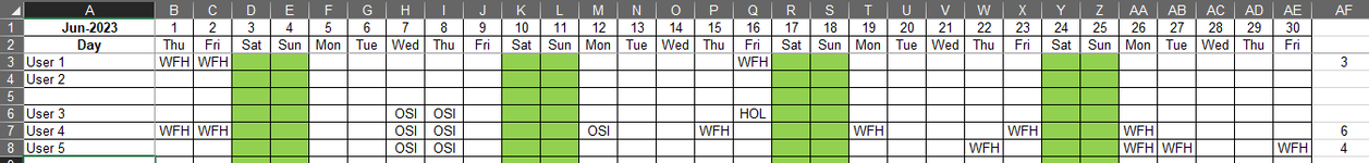
We have a planner as such, which identifies when people are on holiday (HOL), working from home (WFH), offsite at customers etc (OSI). The working from home is supposed to be on a random pattern and not on a regular day etc, but I have no intention of closely managing this. However a quick glance over a month by month view of the total days people are at home with give me a clue. ie if they are off every Friday, there's a pattern. Its going to be crude, but it will give me something to defend the department with.
Anyway, i have created a formula that works something like this:
1. Looks at the user row for the value WFH.
2. Looks at the top row for the day (ie Mon/Tue..etc)
3. Sums the values.
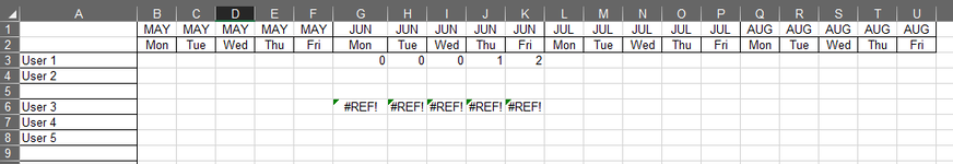
This works fine for user 1. But if I copy down to user 2 I get a REF! error and I cannot figure out why.
This is my formula:
=COUNTIFS(JUN!$B$3:$AE$3,"WFH",INDEX(JUN!$B$2:$AE$2,MATCH($A3,JUN!$A$3:$A$33,0),0),G$2)
For info I have monthly tabs, so the goal is to set it up such that it looks at each individual tab.
I would appreciate your thoughts!
Many thanks,
Jason
We have a planner as such, which identifies when people are on holiday (HOL), working from home (WFH), offsite at customers etc (OSI). The working from home is supposed to be on a random pattern and not on a regular day etc, but I have no intention of closely managing this. However a quick glance over a month by month view of the total days people are at home with give me a clue. ie if they are off every Friday, there's a pattern. Its going to be crude, but it will give me something to defend the department with.
Anyway, i have created a formula that works something like this:
1. Looks at the user row for the value WFH.
2. Looks at the top row for the day (ie Mon/Tue..etc)
3. Sums the values.
This works fine for user 1. But if I copy down to user 2 I get a REF! error and I cannot figure out why.
This is my formula:
=COUNTIFS(JUN!$B$3:$AE$3,"WFH",INDEX(JUN!$B$2:$AE$2,MATCH($A3,JUN!$A$3:$A$33,0),0),G$2)
For info I have monthly tabs, so the goal is to set it up such that it looks at each individual tab.
I would appreciate your thoughts!
Many thanks,
Jason