Conditional Formatting Borders

[cjm205]

Does anyone know how to make thicker borders using the Conditional Formatting option? The options they give you are all thin borders.

 

[AlbertanFireFly]

What does your data set look like, and what condition are you trying to format?
For example: if cell B3 is greater than 2, turn cell D3 yellow.
Select cell D3, then click on Conditional Formatting (Home tab), then click New Rule. Under Rule Type click "Use a formula to determine which cells to format", then in the formula box, type =B3>2. Then click Format, and in the Fill tab, click yellow. Click Ok, and OK again.

 

[gcon22]

Hi, this is my sample. I designated a box so that when I type in something, it highlights the whole row that contains what's in that box.

This is the formula I used:
=IF(ISBLANK($B$7), 0, SEARCH($B$7,$A2&$B2&$C2&$D2))

I would like to have regular borders, and have the highlighted section be thick borders if possible.

Thanks!

 

[AlbertanFireFly]

In B7, are you only going to be using the values from the A column, bsbc, bsab, etc. Or are you going to be say inputting 1, and having rows 2, 4 and 5 highlight?

 

[AlbertanFireFly]

As was mentioned earlier, there is no direct way to use thick borders. The work around, is to set the borders to thick as default, and then use conditional formatting to set the borders to thin for all the "false" conditions. Because you want your "true" condition to have both top and bottom borders, this means you're going to end up needing multiple "false" conditions.

Firstly, set all borders to thin if B7 is empty. The formula here is pretty basic:
=ISBLANK($B$7)
and set the format to outline with thin borders.

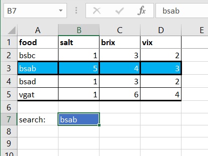
Next bottom borders. Say you have bsab in B7, row 3 is highlighted, so you want rows 4 and 5 to have thin bottom borders, but you want row 2 and 3 to have thick bottom borders. Formula:
=AND(ISERROR(IF(ISBLANK($B$7), 0, SEARCH($B$7,$A2&$B2&$C2&$D2))),ISERROR(IF(ISBLANK($B$7), 0, SEARCH($B$7,$A3&$B3&$C3&$D3))))
and set the format to thin left, right, and bottom borders.

Next top borders. Still with bsab, you want rows 2 and 5 to have thin top borders, but rows 3 and 4 to have thick top borders. Formula:
=AND(ISERROR(IF(ISBLANK($B$7), 0, SEARCH($B$7,$A2&$B2&$C2&$D2))),ISERROR(IF(ISBLANK($B$7), 0, SEARCH($B$7,$A1&$B1&$C1&$D1))))
and set the format to thin left, right, and top borders.

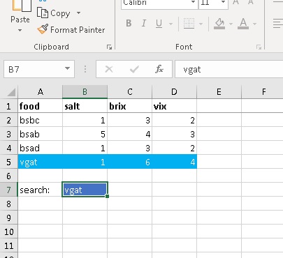
And finally, say you put 1 in B7, and rows 2, 4, and 5 highlight in blue. You want all the top and bottom borders to be bold, but want the left and right borders of row 3 to be thin. Formula:
=ISERROR(IF(ISBLANK($B$7), 0, SEARCH($B$7,$A2&$B2&$C2&$D2)))
and set the format to thin left and right borders.

 

[gcon22]

Wow! It's like magic! Thank you so much! One thing though, how do I get rid of the thick border all the way at the bottom of the data set? Please see image.

Also, what would I need to change in the formula if I did not want thick borders around highlighted rows, but still wanted to retain thin borders around all cells?

Thanks.

 

[Jasesair]

Barry Katcher appears to be helping again, 18 years later! I am using a countifs formula for my desired result to format. I'm now needing a way to do the opposite to try the Barry Katcher work-around. Any ideas?

 

[smallfish]

First, format thick borders around the entire range of those cells you want, then conditional format those cells with "cell value is" "not equal to" or "less than", etc., etc. the criteria you DO NOT WANT with a border, and set the border format to "None".

Barry,

Thank you so much for this helpful suggestion. I came to this thread looking for the same information as the original poster and your solution worked perfectly.

 

[BootieCalls]

Over 20 years later and Mr. Katcher's advice still holds. Unfortunately, Microsoft has yet to add thick borders to conditional formatting.