Conditional Formatting cells with with formula if cells are not blank

[RoryJ80]

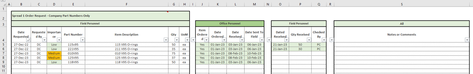
As per the snippet below, I have an internal order spreadsheet set up for our office and field personnel. So they fill out the Field Personnel Columns B to H, I fill out columns J to M and then once the items have arrived to there field location they fill out columns O to Q. I have set up Conditional formatting so that we can see when items have been ordered and sent in in columns J to M and O to Q when is arrived in the field.

What I would like to do and I'm struggling to is add a Conditional Formatting to Columns B to H when a date is added to Column O. So when the field personnel receive the items in the field and add a date to column O it will highlight columns B to H, as in the first snippet below.

In the next snippet, shows the formula I used to be able to highlight those columns in B to H in row 5 but when i try to change the formula so that it will do all rows in column below row 5 i keep getting errors. The spreadsheet row s are infinite there is no end row.

Is there a way so that when the guys in the field add a date to column O it will highlight columns B to H in that particular row?

 

[awoohaw]

Try this:

Book1
	A	B	C	D	E	F	G	H	I	J					O	P
1		ColumnB	ColumnC	ColumnD	ColumnE	ColumnF	ColumnG	ColumnH							ColumnO
2		ZLE	XRT	NRM	XCZ	DLU	APN	MIT							2023-03-14
3		SLH	LSJ	XCM	PKJ	RZE	NLR	FFA							2023-03-18
4		FQO	TEE	YMC	HBX	SUP	KUF	TWJ
5		NEB	NAV	JYL	YCX	DHY	NIX	ZLV
6		SKE	XWN	ZWR	ODN	MNO	YPX	ZWS							2023-03-02
7
Sheet2

Cells with Conditional Formatting
Cell	Condition		Cell Format	Stop If True
B3:H6	Expression	=ISNUMBER($O3)	text	NO
B2:H2	Expression	=ISNUMBER($O2)	text	NO

 

[RoryJ80]

I tried this and it didnt change the columns B to H

 

[awoohaw]

why is the "Stop if True"? It probably doesn't make a difference, though.

but, your formula is O in row 3, and youre asking it to apply to B:H in row 5. Is that what you want?

 

[Fluff]

You can use

=$O5<>""

and for the applies to range use something like

=$B$5:$H$5000

 

[RoryJ80]

Thanks Fluff! That worked for me in this spreadsheet

 

[Fluff]

Glad we could help & thanks for the feedback.