Conditional Formatting

mystic19

New Member
Joined
Apr 27, 2024
Messages
3
Office Version
  1. 365
Platform
  1. Windows
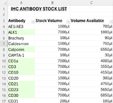
Hi, i'm quite new to excel and wanting to learn and understand it better. I'm struggling on how to conditional format the "Volume Available" column. Ideally what I want is for the cells to be highlighted a colour such as orange if it is less than 20% than the total volume. This is shown in the "Stock Volume" column.

If anyone can suggest a way to link the two column together that would be great or advise another solution. Thanks!
 

Attachments

  • Screenshot 2024-04-27 235958.png
    Screenshot 2024-04-27 235958.png
    48.2 KB · Views: 6

Excel Facts

Did you know Excel offers Filter by Selection?
Add the AutoFilter icon to the Quick Access Toolbar. Select a cell containing Apple, click AutoFilter, and you will get all rows with Apple
1. Select all the numbers in col. C starting from row 4.
2. In the Home tab, click on 'Conditional Formatting'. From the drop down menu, select "New Rule".
3. In the new window that pops up, select: "Use a formula to determine which cells to format"
4. In the box below that, type in the following formula.
=C2/B2<.2
5. Next click on the 'Format' button.
6. Choose whatever color you want.
7. Click OK on your way out.

Screenshot as an example:

Excel new formatting rule.png
 
Upvote 0
deally what I want is for the cells to be highlighted a colour such as orange if it is less than 20% than the total volume. This is shown in the "Stock Volume" column.

Possibly something like this.
Book1
ABC
1IHC ANTIBODY STOCK LIST
2AnitbodyStock VolumeVolume available
3tigellus1000uL700uL
4paralalia1000uL130uL
5llanero7000uL4690uL
6kwarterka1000uL110uL
7toxone1000uL340uL
8interhyal1000uL80uL
9wingcut1000uL750uL
10mattapony7000uL1050uL
11heartdeep7000uL5250uL
12bellwind1000uL100uL
13melipona1000uL380uL
14vestryize7000uL560uL
15seroon7000uL2800uL
16reburden7000uL1050uL
17thiazide1000uL410uL
18ingan7000uL700uL
19sestine7000uL2660uL
20upwork7000uL2870uL
21downlast1000uL290uL
Sheet5
Cells with Conditional Formatting
CellConditionCell FormatStop If True
A3:A21Expression=VALUE(LEFT(C3,LEN(C3)-2))<VALUE(LEFT(B3,LEN(B3)-2))*20/100textNO
 
Upvote 0
The OP said he wants to format col. C labeled as "Volume Available".
 
Upvote 0
1. Select all the numbers in col. C starting from row 4.
2. In the Home tab, click on 'Conditional Formatting'. From the drop down menu, select "New Rule".
3. In the new window that pops up, select: "Use a formula to determine which cells to format"
4. In the box below that, type in the following formula.
=C2/B2<.2
5. Next click on the 'Format' button.
6. Choose whatever color you want.
7. Click OK on your way out.

Screenshot as an example:

View attachment 110605
That worked perfectly! Thank you very much! Much appreciated! :)
 
Upvote 0

Forum statistics

Threads
1,215,741
Messages
6,126,592
Members
449,320
Latest member
Antonino90

We've detected that you are using an adblocker.

We have a great community of people providing Excel help here, but the hosting costs are enormous. You can help keep this site running by allowing ads on MrExcel.com.
Allow Ads at MrExcel

Which adblocker are you using?

Disable AdBlock

Follow these easy steps to disable AdBlock

1)Click on the icon in the browser’s toolbar.
2)Click on the icon in the browser’s toolbar.
2)Click on the "Pause on this site" option.
Go back

Disable AdBlock Plus

Follow these easy steps to disable AdBlock Plus

1)Click on the icon in the browser’s toolbar.
2)Click on the toggle to disable it for "mrexcel.com".
Go back

Disable uBlock Origin

Follow these easy steps to disable uBlock Origin

1)Click on the icon in the browser’s toolbar.
2)Click on the "Power" button.
3)Click on the "Refresh" button.
Go back

Disable uBlock

Follow these easy steps to disable uBlock

1)Click on the icon in the browser’s toolbar.
2)Click on the "Power" button.
3)Click on the "Refresh" button.
Go back
Back
Top