Conditionally formatting a row using a colour scale based on one cell's percentage

[Kato]

Hi Everyone,

I've searched high and low and can't seem to find anyone who has asked this question, let alone any solutions. I'm thinking that it would be a fairly common sort of implementation though so I've probably overlooked something obvious.

I'm using Excel 2007.

My spreadsheet looks something like:

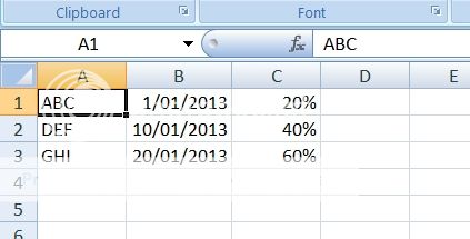
Ideally, I would like to conditionally format a row with a three colour scale based on the percentage in Column C. I've applied conditional formatting across multiple cells before, but never with a colour scale. I'm thinking that the colour scale is my undoing at the moment. I'd prefer a solution that doesn't involve macros because of Excel's security paranoia, not something I really want to deal with in an office environment.

Cheers,

Andy

 

[Snakehips]

Andy,

Welcome to the board.

Two possibilities here.

1 Use the inbuilt CF feature for cells based on percentages. as per example below cells 123.

Conditional formatting > New Rule > Format cells based on their values > select format style
select percentages from the Type dropdown > select values > select colour scale

This will enable you to have 3 colour formatting but I think only in cells that contain a %value.

2 if you want several cells in row formatted based on % in key cells then apply custom format formulas similar to example below cells 456.

Summary

*	B	C	D
1	*	20%	*
2	*	40%	*
3	*	50%	*
4	*	99%	*
5	*	20%	*
6	*	60%	*

<TBODY>
</TBODY>

Conditional formatting

Cell Nr.: / Condition Format C1 1. / Color Scale Abc C2 1. / Color Scale Abc C3 1. / Color Scale Abc C4 1. / Formula is =$C4>66% Abc C4 2. / Formula is =$C4<33% Abc C4 3. / Formula is =$C4<66% Abc C5 1. / Formula is =$C4>66% Abc C5 2. / Formula is =$C4<33% Abc C5 3. / Formula is =$C4<66% Abc C6 1. / Formula is =$C4>66% Abc C6 2. / Formula is =$C4<33% Abc C6 3. / Formula is =$C4<66% Abc <TBODY> </TBODY>

<TBODY>
</TBODY>

Excel tables to the web >> Excel Jeanie Html" target="_blank"> Excel Jeanie HTML 4




Hope that helps

 

[Kato]

Thanks Tony, I was aware of the solutions you posted as they were going to be my fallback option. The percentages along side the data are actually rather inconsequential in the overall scheme of things, in that I was going to implement them to determine the shade of colour used to fill the background of the cells which do actually contain the information that I'm trying to convey. I do find the conditional formatting dialogue box to be quite hamstrung in its application, it's nearly as if the devs thought it would be a good idea to include 'something', but the implementation seems convoluted yet quite restrictive when compared to other Excel features. I wonder if it has been improved on later versions of Excel?

Thank you for your suggestion though.

Cheers,

And

 

[rwatchison4]

Hi Tony,

I'm a newbie here so I hope I can articulate my question well enough.

Here is the scenario, I'm working on a sheet with the same sort of Condition Formatting as above for the most part. We have a document that needs the same kind of color coded ranking. Example: B1 - M1 has Jan. through Dec. respectively which occurs every other row for 224 rows. A2 -A224 (every other row) contains a fish species name (example-Red Grouper). Finally, B2-M2 contain numbers of catch per species per month. Recurring every other row as I hope I explained well enough since I can't seem to attach a screenshot.

The dilemma, I can Format each line showing low to highest number based on the three color coding option. What I would like to do is have this ranking happen for every species row however I can't seem to figure out the correct method and formula since each row is separated by text and finding a way to have each row rank separately from the rest.

What I have been able to do is rank all the numbers but basically the color coding is based on low to highest for every single row with number values rather than individual rows.

I'm so close. I just need to make it do what it's doing but for each individual row with the numbers under each month. This is going to be a new document for each region in the country so you can imagine I don't want to have to format 224 rows 250 times multiple times a year.

I can send the document or screenshot if it would help. The first row shows how it should look for each row relevant.

Any ideas? Thanks ahead of time.

Bobby

 

[Snakehips]

Bobby,

Welcome to MrExcel.

Try this....

Format row 2 to give your required conditional format.
Then select cells B1:M2.
Click the Format Painter icon (paint brush).
Then select cells B3:M??? ??? being as far down the sheet as you wish.
Any rows below, without actual data should show as normal format so you can extend the formatting to the max expected row for data.

That will give you alternate row formatting.
Keep a data-less copy of the sheet to use as a template?

Hope that helps.

 

[rwatchison4]

Bobby,

Welcome to MrExcel.

Try this....

Format row 2 to give your required conditional format.
Then select cells B1:M2.
Click the Format Painter icon (paint brush).
Then select cells B3:M??? ??? being as far down the sheet as you wish.
Any rows below, without actual data should show as normal format so you can extend the formatting to the max expected row for data.

That will give you alternate row formatting.
Keep a data-less copy of the sheet to use as a template?

Hope that helps.

That did it. I have a template and am making all of the necessary regional worksheets thanks to you! Cheers! Bobby

 

[Chaiy]

I have a very similar problem. I have a dataset of used vehicles, with columns for details (year, mileage, make, location etc). The items must be sorted based on what county the vehicle is in. I would need to use the colour scales to visually compare mileage on the vehicles. I would only be using the data from the "mileage" column, but I need the colour scale to apply to the entire row, not just to the single cell within the row.

The colour scale keeps recalculating in all of the numerical rows (i.e. the columns for year, price etc are changing the color scale).

Could anyone suggest a solution. Any help would be appreciated.

 

[Snakehips]

Chaly,

Try something along these lines......
eg 0 to 40,000 = green 40001 to 60000 = amber 60,001 + = red
Mileage in column C
Requires three custom CF formulas in the order shown. The absolute reference to column C, $C, makes sure that it only bases the formatting on the mileage.
Extend the Applies To range to highlight full rows if you wish otherwise just keep top the width of your data.

Excel Workbook
	A	B	C	D	E	F	G
1	Year	Make	Mileage	Location	Price	Stuff	More Stuff
2	2010		52000	East	1000	a	x
3	2011		46000	East	1000	a	x
4	2012		25000	West	1000	a	x
5	2013		60866	North	1000	a	x
6	2014		37000	North	1000	a	x
7	2015		53000	South	1000	b	z
8
9
10
Sheet2

Cells with Conditional Formatting
Cell	Condition		Cell Format	Stop If True
A2	1. / Formula is =$C2>60000	Abc
A2	2. / Formula is =$C2>40000	Abc
A2	3. / Formula is =$C2>0	Abc

Hope that helps.

 

[ArtemL]

Hi, Chaiy and everyone!

I also searched for the same thing.. This is the only good information about it, but I could'n find even there a solution. Then I decided to construct a VBA macro that would do this job. Based on this vba code (vba - Excel - Copy Conditional Formatting, Remove Rules, Keep Format - Stack Overflow) I reworked it so that it could format one range (range1) based on conditional formating with colour scale applied to another range (range2).

When you apply cond. formating to range2 you should define the beginnings of range1 and range2 with names (ctrl+f3): top left cell of range 1 - condform_start_outp, top left cell of range 2 - condform_start_inp. Then you should copy the following code to new module

Sub condform_colscale_othrng()

i0 = Range("condform_start_outp").Row 'top left cell of range 1
j0 = Range("condform_start_outp").Column + 1

i1 = Range("condform_start_inp").Row 'top left cell of range 2
j1 = Range("condform_start_inp").Column + 1

k = i1 - i0

For i = i0 To i0 + 12 '12 - is the number of rows in range 1 and range 2
For j = j0 To j0 + 14 '14 - number of columns in range1 and range2
'copying formating from range2 to range1
Cells(i, j).Font.FontStyle = Cells(i + k, j).DisplayFormat.Font.FontStyle
Cells(i, j).Interior.Color = Cells(i + k, j).DisplayFormat.Interior.Color
Cells(i, j).Font.Strikethrough = Cells(i + k, j).DisplayFormat.Font.Strikethrough
Next j
Next i

Run the macro and that's all. Hope I'll help someone)

Kind regards, AryomL
Moscow

p.s. this is my first post, so don't judge me))