Connect periods with spilled result, where the result is same as the calculated result in previous row

[roelandwatteeuw]

Hi all

Thanks for taking time to read my problem.

Let me first quickly introduce you to the data.

Data:

The black columns are given data:

A - Number: Is an unique number per product​

B - Begin: Start date from the product​

C - End: End date from the product​

This data is sorted:

First on column A - Number: Low to High​

Next on column B - Begin: Low to High​

​

The green and orange columns are calculated ones:

D - Abegin: Connects the periods if they directly follow each other AND have the same number​

E - Key: Concatinates the 'Number' and 'Abegin'​

F - Aend: Gives the maximum value from column C - End, when the key matches the key of the current row​

Used Formulas:

​

D	E	F
Abegin	Key	Aend
=IF( ISNUMBER($B1); IF( AND($A2 = $A1; $B2 = $C1+1); $D1; $B2 ); $B2 )	=$A2 & "-" & $D2	=MAXIFS( $C:$C; $E:$E; $E2 )
If the the cell in column B, from the row above isn't a number, then give the begin date from the current row (this is to avoid an error on the first row) If the cel is a number, then look in row above to the end date. If that end date is exactly one day before the Begin date from the current row, then take the result that was calculated in the row above. If not, then give the begin date from the currect row	Putting 'Number' and 'Begin' together	Gives the max. value from 'End' if the key matches

Problem:

These formulas work great... so where's the problem?
I want to use them as a spilled result.

The 'Key' and 'Aend' columns aren't a problem, but the 'Abegin' is.
I can't find a way to get the calculated result from the row above.
Probably need a LAMBDA or something...


My current formula for Abegin is:

=IF( ISNUMBER( OFFSET(lst_Begin; -1; 0) ); IF( (lst_Nr = lst_NrPrev) * ( lst_Begin = OFFSET(lst_Begin; -1; 1)+1 ); "PREV DATE"; lst_Begin ); lst_Begin )

lst_Begin = all data from column B - Begin - without header (B2:B10) lst_Nr = all data from column A - Number - without header (A2:A10) lst_NrPrev = Number in the previous row (A1:A9)

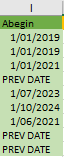
Result with this formula is in column I:

So I need a formula that fills in the 'PREV DATE' value.

If needed, I can upload the file.

thx!

Grtz
Roeland

 

[Fluff]

How about

=DROP(REDUCE("",A2:A10,LAMBDA(x,y,VSTACK(x,MIN(FILTER(B2:B10,A2:A10=y))))),1)

 

[roelandwatteeuw]

How about

=DROP(REDUCE("",A2:A10,LAMBDA(x,y,VSTACK(x,MIN(FILTER(B2:B10,A2:A10=y))))),1)

Hi Fluff

Thought it looked good, but it can only connect to directly following period
In row 6 en 7 this isn't the case, so the result in row 7 can't be the same as the one in row 6.

But it looks like were on the good way

 

[Fluff]

If col B has to be the following month from Col C, I would stick with a drag down formula.

 

[roelandwatteeuw]

If col B has to be the following month from Col C, I would stick with a drag down formula.

Not only the next month, but also the next day.

Hmm... I want to get rid off the drag down formula, because the column is part off many more calculations to come... and it's the only formula that I can't change into a spilled result.
So it would really fasten the proces and avoid errors (if the result is longer and I forget to drag it all the way down...)

But thanks anyway for your help, Fluff

 

[Fluff]

You could try

=DROP(REDUCE("",SEQUENCE(ROWS(A2:A10)),LAMBDA(x,y,VSTACK(x,IF(y=1,INDEX(B2:B10,y),IF(AND(INDEX(A2:A10,y)=INDEX(A2:A10,y-1),INDEX(C2:C10,y-1)+1=INDEX(B2:B10,y)),INDEX(B2:B10,y-1),INDEX(B2:B10,y)))))),1)

 

[roelandwatteeuw]

You could try

=DROP(REDUCE("",SEQUENCE(ROWS(A2:A10)),LAMBDA(x,y,VSTACK(x,IF(y=1,INDEX(B2:B10,y),IF(AND(INDEX(A2:A10,y)=INDEX(A2:A10,y-1),INDEX(C2:C10,y-1)+1=INDEX(B2:B10,y)),INDEX(B2:B10,y-1),INDEX(B2:B10,y)))))),1)

Nice Fluff, you're shaking the formulas out off your magical hat.
I'm trying to understand it all, but I think I'll need to dig deeper into the Lambda-function first.

But still not there yet... Getting closer...
The Numbers with 2 lines are perfect, but those with 3 or more rows are still getting the wrong value.

This part "INDEX(B2:B10; y-1)" should be "INDEX(O2:O10; y-1)" (if used in O2), but that would give a circular reference.

Pff... hard, maybe it's not possible... but I hope it is.

 

[Fluff]

This part "INDEX(B2:B10; y-1)" should be "INDEX(O2:O10; y-1)" (if used in O2)

No, it still needs to be col B regardless of where you put the formula.

 

[roelandwatteeuw]

I tried something different

I've added 2 extra column.
H - Change? : Determine whether the Begin date needs a change (value from above)
I - Nr records up? : Number of rows it has to look up. With this number I can determine the correct row in the 'Begin' column.

All looking good, except when I use more the 2 following periods.
The calculation in column 'I' isn't what it should be.
Column 'I' has to make the sum of colomn 'H', but only for the periods that are connected.
You could say, when there's "-" (zero) in column 'H', counting has to restart in the next row.

In the image above you can see on row '11' had the value "2" in column 'I'.
This should be "3", off course.

Used formulas:

H - Change?	I - Nr records up?	J - Abegin
=( --(lst_Nr = lst_NrPrev) ) * ( IFERROR(--( lst_Begin = ( OFFSET(lst_End; -1; 0) + 1) ); 0) )	=IF( (lst_Nr = lst_NrPrev) * (H2#); H2# + OFFSET(H2#; -1; 0); 0 )	=LET( CountRow; SEQUENCE(ROWS(lst_Nr)); IF(H2#; INDEX(lst_Begin; CountRow - I2#); lst_Begin ) )
Looks up whether the record needs to look up in a row above or not	Counts the number of rows that need to be looked upwards	Searches the number of rows above the current row in the begin date column

lst_Nr = A2:A10
lst_NrPrev = A1:A9
lst_Begin = B2:B10
lst_End = C2:C10


So I'm looking for a way to make the sum of column 'H' for the connected periods.
Maybe this is more possible to work out?

 

[Fluff]

How about

=DROP(REDUCE("",UNIQUE(FILTER(A2:A100,A2:A100<>"")),LAMBDA(x,y,LET(f,FILTER(B2:C100,A2:A100=y),r,VSTACK(99,DROP(INDEX(f,,1),1)-DROP(INDEX(f,,2),-1)),VSTACK(x,IF(ROWS(f)=1,INDEX(f,,1),DROP(REDUCE("", SEQUENCE(ROWS(f)),LAMBDA(m,n,VSTACK(m,INDEX(f,XMATCH(TRUE,CHOOSEROWS(r,SEQUENCE(n))<>1,,-1),1)))),1)))))),1)