Convert formula into code

[RAJESH1960]

Hello experts,
This is JohnnyL's code and I need some help to correct some issues and also add one line of code in the end to update the application.
I have tried to address the issue as simple as possible in the conditions sheet.
The formula to color the cells in the combined data sheet is set for 218 sheets in this file. The range of rows will vary each time from 100 to 20,000 rows in different scenarios. So, instead of writing the code for a fixed range, if the code can count the number of rows in the Combined data sheet it will be really cool.
The formula is for ____Under one Gstin number, in the combined data sheet color rows which have the same amounts repeated more than 2 times this formula color the cells (Color Yellow) from A: N if applied in CF. I have colored manually to show the result.

=SUMPRODUCT(($C$2:$C$218=$C2)*($G$2:$G$218>$G2-1)*($G$2:$G$218<$G2+1)*($H$2:$H$218>$H2-1)*($H$2:$H$218<$H2+1)*($I$2:$I$218>$I2-1)*($I$2:$I$218<$I2+1))>2

Match Portal with 2B.xlsm

 

[johnnyL]

I have made the following changes to correct the coloring:

    With wsMatched
        .Range("A2").Resize(UBound(MatchedArray, 1), UBound(MatchedArray, 2)) = MatchedArray        '   Display results to Matched sheet
'
        For Each Cel In .Range("B2:B" & .Range("B" & Rows.Count).End(xlUp).Row)                     '   Loop through all cells in column B on the Matched sheet
            If Cel.Value = "PORTAL" Then                                                            '       If Cell value is 'PORTAL' then ...
''                Cel.EntireRow.Interior.Color = RGB(146, 208, 80)                                    '           Color the row
''                Cel.EntireRow.Font.Bold = True                                                      '           Bold the row
                .Range("A" & Cel.Row & ":N" & Cel.Row).Interior.Color = RGB(146, 208, 80)           '           Color the columns
                .Range("A" & Cel.Row & ":N" & Cel.Row).Font.Bold = True                             '           Bold the columns
            End If
        Next                                                                                        '   Loop back
    End With
'
    With wsMismatches
        .Range("A2").Resize(UBound(MismatchesArray, 1), UBound(MismatchesArray, 2)) = MismatchesArray   '   Display results to Mismatches sheet
'
        For Each Cel In .Range("B2:B" & .Range("B" & Rows.Count).End(xlUp).Row)                     '   Loop through all cells in column B on the Mismatches sheet
            If Cel.Value = "PORTAL" Then                                                            '       If Cell value is 'PORTAL' then ...
''                Cel.EntireRow.Interior.Color = RGB(146, 208, 80)                                    '           Color the row
''                Cel.EntireRow.Font.Bold = True                                                      '           Bold the row
                .Range("A" & Cel.Row & ":N" & Cel.Row).Interior.Color = RGB(146, 208, 80)           '           Color the columns
                .Range("A" & Cel.Row & ":N" & Cel.Row).Font.Bold = True                             '           Bold the columns
            End If
        Next                                                                                        '   Loop back
    End With

I also made the following change to correct Column O from displaying 'As per purchases':

    With wsDestination
        .Range("A" & DestinationStartRow).Resize(UBound(CorrectedDataArray, _
            1), UBound(CorrectedDataArray, 2)) = CorrectedDataArray                                 ' Display Results to destination sheet
'
        .Range("F:F").NumberFormat = "dd-mm-yyyy"                                                   ' Format the date the way we want it to appear
'
        .Columns("M:M").TextToColumns Destination:=.Range("M1"), _
            DataType:=xlDelimited, FieldInfo:=Array(1, 4)                                           ' Convert text to numeric
'
        DestinationLastRow = .Range("B" & .Rows.Count).End(xlUp).Row                                ' Recalculate last row used in column B of the destination sheeet
'
''        .Range("N" & DestinationStartRow & ":O" & DestinationLastRow) = "As per " & DataWorkSheet   ' Copy 'As Per ' & sheet name to Column O
        .Range("N" & DestinationStartRow & ":N" & DestinationLastRow) = "As per " & DataWorkSheet   ' Copy 'As Per ' & sheet name to Column N
'
        .Range("A" & DestinationStartRow & ":A" & DestinationLastRow).Formula = "=Row() - 1"        ' Use formula to set row #s
        .Range("A" & DestinationStartRow & ":A" & DestinationLastRow).Copy                          ' Copy formula range into memory (clipboard)
        .Range("A" & DestinationStartRow & ":A" & DestinationLastRow).PasteSpecial xlPasteValues    ' Paste just the vales back to range
        Application.CutCopyMode = False                                                             ' Clear clipboard & 'marching ants' around copied range
    End With
End Sub

I honestly don't understand what the rest of your requests are. Perhaps you could rephrase the rest of what you want to happen. which sheet, which cells, etc.

 

[RAJESH1960]

Good Morning JohnnyL,
Both the issues are solved successfully. Thanks man.
The last query is connected to the combined data sheet only. If you check the Combined Data sheet there are rows where under one GSTIN number there are amounts in G, H and I columns, you will notice that the amounts are same and appear more than twice like in rows 2,3,4 and 7,8,9 and 137,138,139, etc.,,. In some cases, there may be amounts which appear 4 or 5 times also. I want to color those rows with yellow color which appear more than twice. The formula to enter in the conditional formatting > new rule is

=SUMPRODUCT(($C$2:$C$218=$C2)*($G$2:$G$218>$G2-1)*($G$2:$G$218<$G2+1)*($H$2:$H$218>$H2-1)*($H$2:$H$218<$H2+1)*($I$2:$I$218>$I2-1)*($I$2:$I$218<$I2+1))>2

If I edit the formula to 20,000 rows, then it will color all the rows below the data which are blank till the count of 20,000 rows.
So, If you write the code in such a way that it applies CF to color the cells with data only not the blank cells.
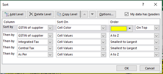
Finally, I want to sort the combined sheet like in the image.

 

[RAJESH1960]

Finally the combined sheet will look like this...

Query Posted Match Portal with 2B.xlsm
	A	B	C	D	E	F	G	H	I	J	K	L	M	N
1	Line	As Per	GSTIN of supplier	Trade/Legal name of the Supplier	Invoice number	Invoice Date	Integrated Tax	Central Tax	State/UT	Remarks	Invoice Value	Taxable Value	Filing Date	Data from
2	112	PORTAL	06AFCPG4749P1Z2		641	11/07/2022	936.00			Matched	8736.00	7800.00	08-11-2022	As Per Portal
3	122	TALLY	06AFCPG4749P1Z2		633	28-06-2022	936.00			Matched	8736.00	7800.00		As per Purchases
4	132	TALLY	06AFCPG4749P1Z2		641	11-07-2022	936.00			Not Found	8736.00	7800.00		As per Purchases
5	7	PORTAL	07AAAPM6196P1Z1		RMO/22-23/170	11/04/2022	993.60			Matched	6514.00	5520.00	05-10-2022	As Per Portal
6	12	PORTAL	07AAAPM6196P1Z1		RMO/22-23/171	11/04/2022	993.60			Not Found	6514.00	5520.00	05-10-2022	As Per Portal
7	163	TALLY	07AAAPM6196P1Z1		RMO	15-04-2022	993.60			Matched	6514.00	5520.40		As per Purchases
8	10	PORTAL	29ABWPS3367H1ZR		GST-0735/22-23	29/04/2022		207.36	207.36	Matched	2719.00	2304.00	05-10-2022	As Per Portal
9	11	PORTAL	29ABWPS3367H1ZR		GST-0736/22-23	29/04/2022		207.36	207.36	Not Found	2719.00	2304.00	05-10-2022	As Per Portal
10	217	TALLY	29ABWPS3367H1ZR		GST-0735	29-04-2022		207.36	207.36	Matched	2719.00	2304.28		As per Purchases
11	13	PORTAL	29AULPB5486A1ZM		22-23/MS-320	22/04/2022		70.20	70.20	Matched	920.00	780.00	05-11-2022	As Per Portal
12	20	PORTAL	29AULPB5486A1ZM		22-23/MS-322	22/04/2022		70.20	70.20	Not Found	920.00	780.00	05-11-2022	As Per Portal
13	182	TALLY	29AULPB5486A1ZM		MS-322	22-04-2022		70.20	70.20	Matched	920.00	779.60		As per Purchases
14	40	PORTAL	07AAAFJ0164C1Z0		2022-23/JK-019	04/04/2022	2673.00			Matched	17523.00	14850.00	05-11-2022	As Per Portal
15	131	TALLY	07AAAFJ0164C1Z0		JK-019	05-04-2022	2673.00			Matched	17523.00	14850.00		As per Purchases
16	54	PORTAL	07AASFP4051E1Z6		2022230153	11/04/2022	2700.00			Matched	17700.00	15000.00	05-11-2022	As Per Portal
17	158	TALLY	07AASFP4051E1Z6		2022230153	12-04-2022	2700.00			Matched	17700.00	15000.00		As per Purchases
18	55	PORTAL	07AASFP4051E1Z6		2022230237	16/04/2022	4608.00			Matched	30208.00	25600.00	05-11-2022	As Per Portal
Combined Data

Cells with Conditional Formatting
Cell	Condition		Cell Format	Stop If True
A2:N229	Expression	=SUMPRODUCT(($C$2:$C$218=$C2)*($G$2:$G$218>$G2-1)*($G$2:$G$218<$G2+1)*($H$2:$H$218>$H2-1)*($H$2:$H$218<$H2+1)*($I$2:$I$218>$I2-1)*($I$2:$I$218<$I2+1))>2	text	NO

 

[RAJESH1960]

I forgot to mention that there may be cases where you may not find same amount rows under one GSTIN number in more than 2 rows. So, add an if condition to the code, if found then color the rows and sort by yellow color else do nothing, just sort the data.

 

[johnnyL]

See if the following does what you are looking for:

Sub Add_CF_FormulaThenSort()
'
    Dim LastRow     As Long
    Dim SortRange   As Range
'
    With Sheets("Combined Data")
        LastRow = .Range("A" & .Rows.Count).End(xlUp).Row
'
        With .Range("A2:N" & LastRow)
            .FormatConditions.Add Type:=xlExpression, Formula1:= _
                    "=SUMPRODUCT(($C$2:$C$" & LastRow & "=$C2)*($G$2:$G$" & LastRow & ">$G2-1)*($G$2:$G$" & LastRow & "<$G2+1)*($H$2:$H$" & _
                    LastRow & ">$H2-1)*($H$2:$H$" & LastRow & "<$H2+1)*($I$2:$I$" & LastRow & ">$I2-1)*($I$2:$I$" & LastRow & "<$I2+1))>2"
'
            .FormatConditions(.FormatConditions.Count).SetFirstPriority
            .FormatConditions(1).Interior.Color = 65535
            .FormatConditions(1).StopIfTrue = False
        End With
    End With
'
'----------------------------------------------------------------------------------------------------------------------------------------------
'
    Set SortRange = Sheets("Combined Data").Range("A2:N" & LastRow)
'
    With Sheets("Combined Data").Sort.SortFields
        .Clear
        .Add(key:=Range("C2"), SortOn:=xlSortOnCellColor, Order:=xlAscending, DataOption:=xlSortNormal).SortOnValue.Color = RGB(255, 255, 0)
        .Add key:=Range("C2"), SortOn:=xlSortOnValues, Order:=xlAscending, DataOption:=xlSortNormal
        .Add key:=Range("G2"), SortOn:=xlSortOnValues, Order:=xlAscending, DataOption:=xlSortNormal
        .Add key:=Range("H2"), SortOn:=xlSortOnValues, Order:=xlAscending, DataOption:=xlSortNormal
        .Add key:=Range("B2"), SortOn:=xlSortOnValues, Order:=xlAscending, DataOption:=xlSortNormal
    End With
'
    With Sheets("Combined Data").Sort
        .SetRange SortRange
        .Apply
    End With
End Sub

 

[RAJESH1960]

Hi @johnnyL , Good Morning

 

[johnnyL]

Hello

 

[RAJESH1960]

In the VBA project I have inserted your module and saved it. In the Match portal where do I insert
call Add_CF_FormulaThenSort..?

 

[johnnyL]

For now, just run that module after all of the sheets have been generated.