Copy column data without blanks and paste into adjacent column WITHOUT deleting cells

[Richard_mcr]

Hello!

I have been looking for a solutions and whilst may come close, none are close enough for my limited VBA knowledge to adapt!

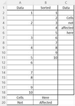
Here is my problem: I have data with random blank cells in column A and I would like to copy the data into column B without the blanks; however, I need to maintain the rows to the right and below.

I have tried to use both the skip blanks and delete blanks, however this affects the adjacent cells / rows.

In the image, you can see the random data in A, and how I would like it in B.

Thank you in advance for any assistance!!

 

[alansidman]

With Power Query

let
    Source = Excel.CurrentWorkbook(){[Name="Table1"]}[Content],
    #"Filtered Rows" = Table.SelectRows(Source, each ([Data] <> null))
in
    #"Filtered Rows"

Data	Data
1	1
	2
2	3
	4
	5
3	6
	7
4	8
	9
5	10
6
7
8
9
10

 

[kevin9999]

VBA Option:

Option Explicit
Sub SortSomeCells()
    Dim ws As Worksheet
    Set ws = Worksheets("Sheet1")       '<-- *** Change to actual sheet name ****
    Dim r As Range, c As Range, LRow As Long, i As Long, a
    LRow = ws.Cells(Rows.Count, "A").End(xlUp).Row
    Set r = ws.Range("A2:A" & LRow)
    ReDim a(1 To LRow, 1 To 1)
    i = 1
    
    For Each c In r
        If c <> "" And IsNumeric(c.Value) Then
            a(i, 1) = c
            i = i + 1
        End If
    Next c
    ws.Range("B2").Resize(i).Value = a
End Sub

 

[Joe4]

Welcome to the Board!

Its too bad you do not have Excel 2021 or 365. This is really easy to do with the new FILTER function.
It would just be this one formula:

=FILTER(A2:A18,A2:A18<>"")

 

[kevin9999]

If your data range in column A is fixed, you could use this:

Sub SortSomeCells_V2()
    Dim ws As Worksheet
    Set ws = Worksheets("Sheet1")       '<-- *** Change to actual sheet name ****
    ws.Range("A2:A18").Copy ws.Range("B2")
    ws.Range("B1:B18").Sort Key1:=ws.Cells(1, 2), _
    order1:=xlAscending, Header:=xlYes
End Sub

 

[MARK858]

A 2019 formula option

Book1 (version 1).xlsb
	A	B
1	Data	2019
2	1	1
3		2
4	2	3
5		4
6		5
7	3	6
8		7
9	4	8
10		9
11	5	10
12	6
13
14	7
15	8
16
17	9
18	10
Sheet6

Cell Formulas
Range	Formula
B2:B12	B2	=IFERROR(INDEX($A$2:$A$18,SMALL(IF($A$2:$A$18<>"",ROW($A$2:$A$18)-ROW($A$2)+1),ROWS($A$2:$A2))),"")

 

[Richard_mcr]

Hi All,

Thank you for the responses, it's much appreciated!

I've gone down Kevin's VBA option!

Happy days!

 

[kevin9999]

Glad we could help & welcome to the board