Copy part of a row from one worksheet to another worksheet based on a cell being updated.

[Kgreen214]

Hi,

I am trying to set this workbook up to create essentially an agenda of items to talk about.

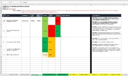
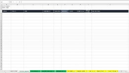
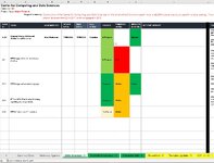
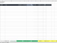
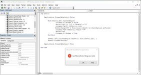
As you can see by the below screenshot I have multiple tabs. Each color tab is different project. I need to copy a row (column A - Column J) from that tab and past in the next available row on the Summary Agenda tab when column I has been updated to via drop down to either Needs Update or Update. I then need the Summary Agenda tab to be sorted in order based on column A(i.e. A.1.1, A1.8, A.2.3, etc.)

 

[vcoolio]

Hello KGreen,

See if this code assigned to a button works for you:-

Sub Test()

    Application.ScreenUpdating = False
    
        With Sheet1.[A7].CurrentRegion
                .AutoFilter 9, "*" & "Update" & "*"
                .Columns("A:J").Offset(1).Copy
                Sheet2.Range("A" & Rows.Count).End(3)(2).PasteSpecial xlValues
                .Columns("A:J").Offset(1).EntireRow.Delete
                .AutoFilter
        End With
        
        Sheet2.[A4].CurrentRegion.Offset(1).Sort Sheet2.[A5], 1
        Sheet2.Columns.AutoFit
        
    Application.ScreenUpdating = True

End Sub

The code only transfers values to the destination sheet as I'd assume that you wouldn't want the formatting to move across as well.
I've used sheet codes (Sheet1 and Sheet2) in this macro, assuming that these are the sheet codes for the source and destination sheets.
To prevent duplication in the destination sheet, I've added a delete line of code as well which will delete the relevant rows from the source sheet once they are transferred to the destination sheet.

I hope that this helps.

Cheerio,
vcoolio.

 

[Kgreen214]

Hello KGreen,

See if this code assigned to a button works for you:-

Sub Test()

    Application.ScreenUpdating = False
   
        With Sheet1.[A7].CurrentRegion
                .AutoFilter 9, "*" & "Update" & "*"
                .Columns("A:J").Offset(1).Copy
                Sheet2.Range("A" & Rows.Count).End(3)(2).PasteSpecial xlValues
                .Columns("A:J").Offset(1).EntireRow.Delete
                .AutoFilter
        End With
       
        Sheet2.[A4].CurrentRegion.Offset(1).Sort Sheet2.[A5], 1
        Sheet2.Columns.AutoFit
       
    Application.ScreenUpdating = True

End Sub

The code only transfers values to the destination sheet as I'd assume that you wouldn't want the formatting to move across as well.
I've used sheet codes (Sheet1 and Sheet2) in this macro, assuming that these are the sheet codes for the source and destination sheets.
To prevent duplication in the destination sheet, I've added a delete line of code as well which will delete the relevant rows from the source sheet once they are transferred to the destination sheet.

I hope that this helps.

Cheerio,
vcoolio.

Hello,

Thanks for this. I actually need a little more help. I would say the values transferring should be fine as the cells themselves have conditional formatting set up so they essentially change colors based on the value in them. But what I do need is for the source sheet row not to be deleted but instead the "update status" column in the source tab to change to having no value in it and everything else remaining the same once the row has been copied over to the summary agenda tab. Hope this makes sense. Thanks!

 

[vcoolio]

Hello KGreen,

In the code supplied, replace this line:-

.Columns("A:J").Offset(1).EntireRow.Delete

with

.Columns("I").Offset(1).Value = ""

This will prevent deletion and remove the "Status" values from the source sheet once the data transfer is done.

I hope that this helps.

Cheerio,
vcoolio.

 

[Kgreen214]

Hi Vcoolio,

I hope all is well. I am reaching back out because I am having some trouble with the code you provided. When I added a column and updated the code to reflect for some reason it no longer wanted to work. Can you assist me with this? Not sure what I'm doing wrong on this one. I've attached the screenshot of the two tabs again for your reference.

Karl

 

[vcoolio]

Hello Karl,

Is the column that you want to add the next column along (Column K) or is it an isolated column further along (e.g. Column P)?

Cheerio,
vcoolio.

 

[Kgreen214]

Hello Karl,

Is the column that you want to add the next column along (Column K) or is it an isolated column further along (e.g. Column P)?

Cheerio,
vcoolio.

Hi Vcoolio,

I inserted a column (column G) which is labeled Date Status. That column actually has a formula which will utilize the date listed in column F to determine if a task is overdue or not. There are no other columns further along then columns M. Thanks again for your help.

 

[Kgreen214]

Hi Vcoolio,

I inserted a column (column G) which is labeled Date Status. That column actually has a formula which will utilize the date listed in column F to determine if a task is overdue or not. There are no other columns further along then columns M. Thanks again for your help.

I don't know if this matters or not there is also a column (column B) that is hidden right now but will need to copy over when using the vba code.

 

[vcoolio]

Hello Karl,

If you've added a column then you've shifted everything one column to the right. This means that the code is no longer filtering on Column 9 ( the original criteria column) but needs to now filter on Column 10. Hence, change the 9 to 10 in this line of code:-

.AutoFilter 9, "*" & "Update" & "*"

You will also need to unhide Column B prior to the filter executing. Hence, add this line of code:

.Columns(2).Hidden = False

directly after this line of code:

With Sheet1.[A7].CurrentRegion

and re-hide Column B after the code has executed by adding this line of code:-

.Columns(2).Hidden = True

directly after:

.AutoFilter

You'll also need to change this line of code:

.Columns("A:J").Offset(1).Copy

to

You'll also need to change this line of code:

.Columns("A:K").Offset(1).Copy

I hope that this helps.

Cheerio,
vcoolio.

 

[Kgreen214]

Hello Karl,

If you've added a column then you've shifted everything one column to the right. This means that the code is no longer filtering on Column 9 ( the original criteria column) but needs to now filter on Column 10. Hence, change the 9 to 10 in this line of code:-

.AutoFilter 9, "*" & "Update" & "*"

You will also need to unhide Column B prior to the filter executing. Hence, add this line of code:

.Columns(2).Hidden = False

directly after this line of code:

With Sheet1.[A7].CurrentRegion

and re-hide Column B after the code has executed by adding this line of code:-

.Columns(2).Hidden = True

directly after:

.AutoFilter

You'll also need to change this line of code:

.Columns("A:J").Offset(1).Copy

to

You'll also need to change this line of code:

.Columns("A:K").Offset(1).Copy

I hope that this helps.

Cheerio,
vcoolio.

Hi Vcoolio,

Unfortunately I got the attached error when I made those updates. (AutoFilter method of Range class failed). Not sure what I'm doing wrong here.