glaccounting
New Member
- Joined
- Jan 4, 2024
- Messages
- 2
- Office Version
- 2016
- Platform
- Windows
Hi All,
I would like to request your help. Not sure if this just needs a simple VBA code, but since I am very new to VBA, this has been giving me problems. Will really appreciate all of you guys help.
Here's the problem. I need to copy range of cells and paste it on the rows below it. But only if it met multiple criteria.
Currently, I have a data (combination of formulas & alphanumeric values) in B13:I17 and L13&L17. In this range, not all of it is filled up. Only certain parts of it contains data.
I also have another table within the sheet that contains the criteria references (range B62:E72).
1st Criteria - Cell L17 formula to be copied and pasted from Cell L18 until 1 Row before the Grand Total Rows (B59:N59) which would be until Cell L57.
2nd Criteria - If cell D67=0 then do nothing, if its D67>0, Range B13:I17 needs to be copied below rows. Formulas to be pasted as formulas, values to be pasted as values. However, there is one cell in the range which is an array formula that needs to be copied and pasted as values which is Cell D13. The number of times range B13:I17 needs to be copied should be equal to the value of D67.
3rd Criteria - If cell D68=0 then Range B13:I17 needs to be copied to the first available blank rows in column B. This time, there is no need for Cell D13 to be pasted as value. All formulas to be copied as formulas, all values to be copied as values as is.
If cell D68>0, then Range B13:I17 needs to be copied to the first available blank rows in column B. This time, there is no need for Cell D13 to be pasted as value. All formulas to be copied as formulas, all values to be copied as values as is. Additionally, D68 value would be set as the number of times of additional copying of Range B13:I17 to the next available blanks rows in Column B with Cell D13 to be pasted as value and not formula.
Do this rule for all the remaining non blank rows for range D68:D71.
After the above, save the file as .pdf - print Area - Range B1:N59
Then, revert the worksheet back to its original untouched form.
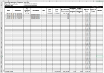
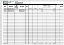
Here is a look of the initial worksheet.
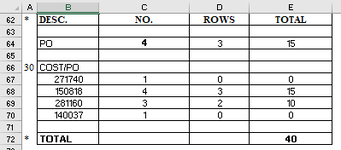
Criteria Reference Table
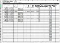
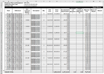
and the finished output.
I would like to request your help. Not sure if this just needs a simple VBA code, but since I am very new to VBA, this has been giving me problems. Will really appreciate all of you guys help.
Here's the problem. I need to copy range of cells and paste it on the rows below it. But only if it met multiple criteria.
Currently, I have a data (combination of formulas & alphanumeric values) in B13:I17 and L13&L17. In this range, not all of it is filled up. Only certain parts of it contains data.
I also have another table within the sheet that contains the criteria references (range B62:E72).
1st Criteria - Cell L17 formula to be copied and pasted from Cell L18 until 1 Row before the Grand Total Rows (B59:N59) which would be until Cell L57.
2nd Criteria - If cell D67=0 then do nothing, if its D67>0, Range B13:I17 needs to be copied below rows. Formulas to be pasted as formulas, values to be pasted as values. However, there is one cell in the range which is an array formula that needs to be copied and pasted as values which is Cell D13. The number of times range B13:I17 needs to be copied should be equal to the value of D67.
3rd Criteria - If cell D68=0 then Range B13:I17 needs to be copied to the first available blank rows in column B. This time, there is no need for Cell D13 to be pasted as value. All formulas to be copied as formulas, all values to be copied as values as is.
If cell D68>0, then Range B13:I17 needs to be copied to the first available blank rows in column B. This time, there is no need for Cell D13 to be pasted as value. All formulas to be copied as formulas, all values to be copied as values as is. Additionally, D68 value would be set as the number of times of additional copying of Range B13:I17 to the next available blanks rows in Column B with Cell D13 to be pasted as value and not formula.
Do this rule for all the remaining non blank rows for range D68:D71.
After the above, save the file as .pdf - print Area - Range B1:N59
Then, revert the worksheet back to its original untouched form.
Here is a look of the initial worksheet.
| OTC Sample Sheet v9.xlsm | |||||||||||||||
|---|---|---|---|---|---|---|---|---|---|---|---|---|---|---|---|
| B | C | D | E | F | G | H | I | J | K | L | M | N | |||
| 11 | Repair History | ||||||||||||||
| 12 | Date | Reference | PO-Contract Number | Description | Qty. | Unit Cost | Total Cost | Accumulated Depreciation | Accumulated Impairment Losses | Issues/ Transfers/ Adjustment/s | Adjusted Cost | Nature of Repair | Amount | ||
| 13 | 08-Apr-08 | JAP-08-04-000045 | 271740 | 3 | 58,500.00 | 175,500.00 | -166,725.00 | 8,775.00 | |||||||
| 14 | 31-Aug-23 | JGL-23-08-000258 | DEPRECIATION | 0.00 | 8,775.00 | ||||||||||
| 15 | 30-Sep-23 | JGL-23-09-000280 | DEPRECIATION | 0.00 | 8,775.00 | ||||||||||
| 16 | 31-Oct-23 | JGL-23-10-000249 | DEPRECIATION | 0.00 | 8,775.00 | ||||||||||
| 17 | 30-Nov-23 | JGL-23-11-000273 | DEPRECIATION | 0.00 | 8,775.00 | ||||||||||
| 18 | |||||||||||||||
| 19 | |||||||||||||||
| 20 | |||||||||||||||
| 21 | |||||||||||||||
| 22 | |||||||||||||||
| 23 | |||||||||||||||
| 24 | |||||||||||||||
| 25 | |||||||||||||||
| 26 | |||||||||||||||
| 27 | |||||||||||||||
| 28 | |||||||||||||||
| 29 | |||||||||||||||
| 30 | |||||||||||||||
| 31 | |||||||||||||||
| 32 | |||||||||||||||
| 33 | |||||||||||||||
| 34 | |||||||||||||||
| 35 | |||||||||||||||
| 36 | |||||||||||||||
| 37 | |||||||||||||||
| 38 | |||||||||||||||
| 39 | |||||||||||||||
| 40 | |||||||||||||||
| 41 | |||||||||||||||
| 42 | |||||||||||||||
| 43 | |||||||||||||||
| 44 | |||||||||||||||
| 45 | |||||||||||||||
| 46 | |||||||||||||||
| 47 | |||||||||||||||
| 48 | |||||||||||||||
| 49 | |||||||||||||||
| 50 | |||||||||||||||
| 51 | |||||||||||||||
| 52 | |||||||||||||||
| 53 | |||||||||||||||
| 54 | |||||||||||||||
| 55 | |||||||||||||||
| 56 | |||||||||||||||
| 57 | |||||||||||||||
| 58 | |||||||||||||||
| 59 | GRAND TOTAL | 175,500.00 | -166,725.00 | 0.00 | 0.00 | 8,775.00 | |||||||||
Testing (2) | |||||||||||||||
| Cell Formulas | ||
|---|---|---|
| Range | Formula | |
| B13 | B13 | =VLOOKUP(C13,JEV:Tdate,2,FALSE) |
| C13 | C13 | =VLOOKUP(D13,PONUM:(JEV),2,FALSE) |
| D13 | D13 | =IFNA(LOOKUP(2,1/((COUNTIF($D12:D$12,PONUM)=0)*($D$8&$D$9=TYPE&ACCCODE)),PONUM),"") |
| F13 | F13 | =COUNTIFS(COST,G13,TYPE,$D$8,PONUM,$D13) |
| G13 | G13 | =IFERROR(INDEX(COST,MATCH(0,COUNTIF(G12:$G$12,COST)+IF(TYPE<>$D$8,1,0)+IF(PONUM<>$D13,1,0),0)),"") |
| H13 | H13 | =+F13*G13 |
| I13 | I13 | =SUMIFS(BEGDEP,TYPE,$D$8,ACCCODE,$D$9,JEV,$C13,PONUM,$D13,COST,$G13) |
| I14 | I14 | =SUMIFS(BEGDEP,TYPE,$D$8,ACCCODE,$D$9,JEV,$C14,PONUM,D13,COST,G13) |
| I15 | I15 | =SUMIFS(BEGDEP,TYPE,$D$8,ACCCODE,$D$9,JEV,$C15,PONUM,D13,COST,G13) |
| I16 | I16 | =SUMIFS(BEGDEP,TYPE,$D$8,ACCCODE,$D$9,JEV,$C16,PONUM,D13,COST,G13) |
| I17 | I17 | =SUMIFS(BEGDEP,TYPE,$D$8,ACCCODE,$D$9,JEV,$C17,PONUM,D13,COST,G13) |
| L13,L59 | L13 | =SUM(H13:K13) |
| L14:L17 | L14 | =L13+(SUM(H14:K14)) |
| H59:K59 | H59 | =SUBTOTAL(9,H13:H58) |
| Press CTRL+SHIFT+ENTER to enter array formulas. | ||
| Named Ranges | ||
|---|---|---|
| Name | Refers To | Cells |
| Data!_FilterDatabase | =Data!$A$5:$P$30 | I13:I17, D13, F13:G13 |
| ACCCODE | =Data!$B$5:$B$30 | I13:I17, D13 |
| BEGDEP | =Data!$H$5:$H$30 | I13:I17 |
| COST | =Data!$G$5:$G$30 | I13:I17, F13:G13 |
| JEV | =Data!$D$5:$D$30 | I13:I17, B13:C13 |
| PONUM | =Data!$C$5:$C$30 | I13:I17, F13:G13, C13:D13 |
| Tdate | =Data!$E$5:$E$30 | B13 |
| TYPE | =Data!$A$5:$A$30 | I13:I17, D13, F13:G13 |
Criteria Reference Table
| OTC Sample Sheet v9.xlsm | ||||||
|---|---|---|---|---|---|---|
| B | C | D | E | |||
| 62 | DESC. | NO. | ROWS | TOTAL | ||
| 63 | ||||||
| 64 | PO | 4 | 3 | 15 | ||
| 65 | ||||||
| 66 | COST/PO | |||||
| 67 | 271740 | 1 | 0 | 0 | ||
| 68 | 150818 | 4 | 3 | 15 | ||
| 69 | 281160 | 3 | 2 | 10 | ||
| 70 | 140037 | 1 | 0 | 0 | ||
| 71 | ||||||
| 72 | TOTAL | 40 | ||||
Testing (2) | ||||||
| Cell Formulas | ||
|---|---|---|
| Range | Formula | |
| C64 | C64 | =SUM(--(FREQUENCY(IF(PONUM<>"",IF(TYPE=$D$8,IF(ACCCODE=$D$9,MATCH(PONUM,PONUM,0)))),ROW(PONUM)-ROW(Table2[[#Headers],[PO-Contract Number]])+1)>0)) |
| D64,D67:D70 | D64 | =(C64-1) |
| E64,E67:E70 | E64 | =D64*5 |
| B67 | B67 | =IFNA(LOOKUP(2,1/((COUNTIF($B66:B$66,PONUM)=0)*($D$8&$D$9=TYPE&ACCCODE)),PONUM),"") |
| C67:C70 | C67 | =SUM(--(FREQUENCY(IF(COST<>"",IF(TYPE=$D$8,IF(ACCCODE=$D$9,IF(PONUM=$B67,MATCH(COST,COST,0))))),ROW(COST)-ROW(Table2[[#Headers],[Acquisition Cost]])+1)>0)) |
| B68:B70 | B68 | =IFNA(LOOKUP(2,1/((COUNTIF($B$66:B67,PONUM)=0)*($D$8&$D$9=TYPE&ACCCODE)),PONUM),"") |
| E72 | E72 | =SUM(E64:E71) |
| Press CTRL+SHIFT+ENTER to enter array formulas. | ||
| Named Ranges | ||
|---|---|---|
| Name | Refers To | Cells |
| Data!_FilterDatabase | =Data!$A$5:$P$30 | B67:C70, C64 |
| ACCCODE | =Data!$B$5:$B$30 | B67:C70, C64 |
| COST | =Data!$G$5:$G$30 | C67:C70 |
| PONUM | =Data!$C$5:$C$30 | B67:C70, C64 |
| TYPE | =Data!$A$5:$A$30 | B67:C70, C64 |
and the finished output.
| OTC Sample Sheet v9.xlsm | |||||||||||||||
|---|---|---|---|---|---|---|---|---|---|---|---|---|---|---|---|
| B | C | D | E | F | G | H | I | J | K | L | M | N | |||
| 12 | Date | Reference | PO-Contract Number | Description | Qty. | Unit Cost | Total Cost | Accumulated Depreciation | Accumulated Impairment Losses | Issues/ Transfers/ Adjustment/s | Adjusted Cost | Nature of Repair | Amount | ||
| 13 | 08-Apr-08 | JAP-08-04-000045 | 271740 | 3 | 58,500.00 | 175,500.00 | -166,725.00 | 8,775.00 | |||||||
| 14 | 31-Aug-23 | JGL-23-08-000258 | DEPRECIATION | 0.00 | 8,775.00 | ||||||||||
| 15 | 30-Sep-23 | JGL-23-09-000280 | DEPRECIATION | 0.00 | 8,775.00 | ||||||||||
| 16 | 31-Oct-23 | JGL-23-10-000249 | DEPRECIATION | 0.00 | 8,775.00 | ||||||||||
| 17 | 30-Nov-23 | JGL-23-11-000273 | DEPRECIATION | 0.00 | 8,775.00 | ||||||||||
| 18 | 25-Jan-16 | JGL-16-01-000196 | 150818 | 6 | 24,335.00 | 146,010.00 | -138,709.50 | 16,075.50 | |||||||
| 19 | 31-Aug-23 | JGL-23-08-000258 | DEPRECIATION | 0.00 | 16,075.50 | ||||||||||
| 20 | 30-Sep-23 | JGL-23-09-000280 | DEPRECIATION | 0.00 | 16,075.50 | ||||||||||
| 21 | 31-Oct-23 | JGL-23-10-000249 | DEPRECIATION | 0.00 | 16,075.50 | ||||||||||
| 22 | 30-Nov-23 | JGL-23-11-000273 | DEPRECIATION | 0.00 | 16,075.50 | ||||||||||
| 23 | 25-Jan-16 | JGL-16-01-000196 | 150818 | 1 | 25,000.00 | 25,000.00 | -23,750.00 | 17,325.50 | |||||||
| 24 | 31-Aug-23 | JGL-23-08-000258 | DEPRECIATION | 0.00 | 17,325.50 | ||||||||||
| 25 | 30-Sep-23 | JGL-23-09-000280 | DEPRECIATION | 0.00 | 17,325.50 | ||||||||||
| 26 | 31-Oct-23 | JGL-23-10-000249 | DEPRECIATION | 0.00 | 17,325.50 | ||||||||||
| 27 | 30-Nov-23 | JGL-23-11-000273 | DEPRECIATION | 0.00 | 17,325.50 | ||||||||||
| 28 | 25-Jan-16 | JGL-16-01-000196 | 150818 | 1 | 52,390.00 | 52,390.00 | -49,770.50 | 19,945.00 | |||||||
| 29 | 31-Aug-23 | JGL-23-08-000258 | DEPRECIATION | 0.00 | 19,945.00 | ||||||||||
| 30 | 30-Sep-23 | JGL-23-09-000280 | DEPRECIATION | 0.00 | 19,945.00 | ||||||||||
| 31 | 31-Oct-23 | JGL-23-10-000249 | DEPRECIATION | 0.00 | 19,945.00 | ||||||||||
| 32 | 30-Nov-23 | JGL-23-11-000273 | DEPRECIATION | 0.00 | 19,945.00 | ||||||||||
| 33 | 25-Jan-16 | JGL-16-01-000196 | 150818 | 2 | 19,000.00 | 38,000.00 | -36,100.00 | 21,845.00 | |||||||
| 34 | 31-Aug-23 | JGL-23-08-000258 | DEPRECIATION | 0.00 | 21,845.00 | ||||||||||
| 35 | 30-Sep-23 | JGL-23-09-000280 | DEPRECIATION | 0.00 | 21,845.00 | ||||||||||
| 36 | 31-Oct-23 | JGL-23-10-000249 | DEPRECIATION | 0.00 | 21,845.00 | ||||||||||
| 37 | 30-Nov-23 | JGL-23-11-000273 | DEPRECIATION | 0.00 | 21,845.00 | ||||||||||
| 38 | 30-Apr-09 | JAP-09-04-000691 | 281160 | 2 | 100,000.00 | 200,000.00 | -190,000.00 | 31,845.00 | |||||||
| 39 | 31-Aug-23 | JGL-23-08-000258 | DEPRECIATION | 0.00 | 31,845.00 | ||||||||||
| 40 | 30-Sep-23 | JGL-23-09-000280 | DEPRECIATION | 0.00 | 31,845.00 | ||||||||||
| 41 | 31-Oct-23 | JGL-23-10-000249 | DEPRECIATION | 0.00 | 31,845.00 | ||||||||||
| 42 | 30-Nov-23 | JGL-23-11-000273 | DEPRECIATION | 0.00 | 31,845.00 | ||||||||||
| 43 | 30-Apr-09 | JAP-09-04-000691 | 281160 | 3 | 130,000.00 | 390,000.00 | -370,500.00 | 51,345.00 | |||||||
| 44 | 31-Aug-23 | JGL-23-08-000258 | DEPRECIATION | 0.00 | 51,345.00 | ||||||||||
| 45 | 30-Sep-23 | JGL-23-09-000280 | DEPRECIATION | 0.00 | 51,345.00 | ||||||||||
| 46 | 31-Oct-23 | JGL-23-10-000249 | DEPRECIATION | 0.00 | 51,345.00 | ||||||||||
| 47 | 30-Nov-23 | JGL-23-11-000273 | DEPRECIATION | 0.00 | 51,345.00 | ||||||||||
| 48 | 30-Apr-09 | JAP-09-04-000691 | 281160 | 6 | 75,000.00 | 450,000.00 | -427,500.00 | 73,845.00 | |||||||
| 49 | 31-Aug-23 | JGL-23-08-000258 | DEPRECIATION | 0.00 | 73,845.00 | ||||||||||
| 50 | 30-Sep-23 | JGL-23-09-000280 | DEPRECIATION | 0.00 | 73,845.00 | ||||||||||
| 51 | 31-Oct-23 | JGL-23-10-000249 | DEPRECIATION | 0.00 | 73,845.00 | ||||||||||
| 52 | 30-Nov-23 | JGL-23-11-000273 | DEPRECIATION | 0.00 | 73,845.00 | ||||||||||
| 53 | 04-Apr-14 | JAP-14-04-000042 | 140037 | 1 | 88,500.00 | 88,500.00 | -84,075.00 | 78,270.00 | |||||||
| 54 | 31-Aug-23 | JGL-23-08-000258 | DEPRECIATION | 0.00 | 78,270.00 | ||||||||||
| 55 | 30-Sep-23 | JGL-23-09-000280 | DEPRECIATION | 0.00 | 78,270.00 | ||||||||||
| 56 | 31-Oct-23 | JGL-23-10-000249 | DEPRECIATION | 0.00 | 78,270.00 | ||||||||||
| 57 | 30-Nov-23 | JGL-23-11-000273 | DEPRECIATION | 0.00 | 78,270.00 | ||||||||||
| 58 | |||||||||||||||
| 59 | GRAND TOTAL | 1,565,400.00 | -1,487,130.00 | 0.00 | 0.00 | 78,270.00 | |||||||||
Testing (2) | |||||||||||||||
| Cell Formulas | ||
|---|---|---|
| Range | Formula | |
| B13,B53,B48,B43,B38,B33,B28,B23,B18 | B13 | =VLOOKUP(C13,JEV:Tdate,2,FALSE) |
| C13,C53,C48,C43,C38,C33,C28,C23,C18 | C13 | =VLOOKUP(D13,PONUM:(JEV),2,FALSE) |
| D13 | D13 | =IFNA(LOOKUP(2,1/((COUNTIF($D12:D$12,PONUM)=0)*($D$8&$D$9=TYPE&ACCCODE)),PONUM),"") |
| F13,F53,F48,F43,F38,F33,F28,F23,F18 | F13 | =COUNTIFS(COST,G13,TYPE,$D$8,PONUM,$D13) |
| G13 | G13 | =IFERROR(INDEX(COST,MATCH(0,COUNTIF(G12:$G$12,COST)+IF(TYPE<>$D$8,1,0)+IF(PONUM<>$D13,1,0),0)),"") |
| H13,H53,H48,H43,H38,H33,H28,H23,H18 | H13 | =+F13*G13 |
| D18,D53,D38 | D18 | =IFNA(LOOKUP(2,1/((COUNTIF($D$12:D17,PONUM)=0)*($D$8&$D$9=TYPE&ACCCODE)),PONUM),"") |
| G18,G53,G48,G43,G38,G33,G28,G23 | G18 | =IFERROR(INDEX(COST,MATCH(0,COUNTIF(G$12:$G17,COST)+IF(TYPE<>$D$8,1,0)+IF(PONUM<>$D18,1,0),0)),"") |
| I13,I53,I48,I43,I38,I33,I28,I23,I18 | I13 | =SUMIFS(BEGDEP,TYPE,$D$8,ACCCODE,$D$9,JEV,$C13,PONUM,$D13,COST,$G13) |
| I14,I54,I49,I44,I39,I34,I29,I24,I19 | I14 | =SUMIFS(BEGDEP,TYPE,$D$8,ACCCODE,$D$9,JEV,$C14,PONUM,D13,COST,G13) |
| I15,I55,I50,I45,I40,I35,I30,I25,I20 | I15 | =SUMIFS(BEGDEP,TYPE,$D$8,ACCCODE,$D$9,JEV,$C15,PONUM,D13,COST,G13) |
| I16,I56,I51,I46,I41,I36,I31,I26,I21 | I16 | =SUMIFS(BEGDEP,TYPE,$D$8,ACCCODE,$D$9,JEV,$C16,PONUM,D13,COST,G13) |
| I17,I57,I52,I47,I42,I37,I32,I27,I22 | I17 | =SUMIFS(BEGDEP,TYPE,$D$8,ACCCODE,$D$9,JEV,$C17,PONUM,D13,COST,G13) |
| L13,L59 | L13 | =SUM(H13:K13) |
| L14:L57 | L14 | =L13+(SUM(H14:K14)) |
| H59:K59 | H59 | =SUBTOTAL(9,H13:H58) |
| Press CTRL+SHIFT+ENTER to enter array formulas. | ||
| Named Ranges | ||
|---|---|---|
| Name | Refers To | Cells |
| Data!_FilterDatabase | =Data!$A$5:$P$30 | I13:I57, D13, D18, D38, D53, F13:G13, F18:G18, F23:G23, F28:G28, F33:G33, F38:G38, F43:G43, F48:G48, F53:G53 |
| ACCCODE | =Data!$B$5:$B$30 | I13:I57, D13, D18, D38, D53 |
| BEGDEP | =Data!$H$5:$H$30 | I13:I57 |
| COST | =Data!$G$5:$G$30 | I13:I57, F13:G13, F18:G18, F23:G23, F28:G28, F33:G33, F38:G38, F43:G43, F48:G48, F53:G53 |
| JEV | =Data!$D$5:$D$30 | I13:I57, B13:C13, B18:C18, B23:C23, B28:C28, B33:C33, B38:C38, B43:C43, B48:C48, B53:C53 |
| PONUM | =Data!$C$5:$C$30 | I13:I57, F13:G13, F18:G18, F23:G23, F28:G28, F33:G33, F38:G38, F43:G43, F48:G48, F53:G53, C13:D13, C18:D18, C23, C28, C33, C38:D38, C43, C48, C53:D53 |
| Tdate | =Data!$E$5:$E$30 | B13, B18, B23, B28, B33, B38, B43, B48, B53 |
| TYPE | =Data!$A$5:$A$30 | I13:I57, D13, D18, D38, D53, F13:G13, F18:G18, F23:G23, F28:G28, F33:G33, F38:G38, F43:G43, F48:G48, F53:G53 |
Attachments
-
 Initial Worksheet.PNG44.1 KB · Views: 3
 -
 Criteria Reference.PNG5.6 KB · Views: 2
 -
 After 1st Criteria.PNG54.1 KB · Views: 3
 -
 After 2nd Criteria.PNG54.1 KB · Views: 2
 -
 After 3rd Criteria.PNG70.6 KB · Views: 4
 -
 Finished Ouput - Before Saving as PDF.PNG97.1 KB · Views: 2
 -
 Reverting Back to Initial Worksheet.PNG44.1 KB · Views: 2


