glaccounting
New Member
- Joined
- Jan 4, 2024
- Messages
- 2
- Office Version
- 2016
- Platform
- Windows
I would like to ask some help. I am very new to VBA and I would really appreciate a lot if you could lend me a hand.
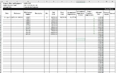
I have 2 Sheets. Output Sheet & Helper Sheet. I want to extract all the values that meets criteria from Helper Sheet, copy all that and paste it to the Output Sheet. And some more additional tasks if you could accommodate.
I would like to copy and paste all the cells from Helper Sheet Column D and Column F over to Output Sheet Column D and G respectively, if OutputSheet Cell D8 & D9 value is equal to the rows of Helper Sheet Column B & C.
After that, I would also like to copy down the formulas in OutputSheet to the last non blank rows of Column D. Notice I already have formulas set up in Cells B13, C13, F13, H13 & I13.
Then paste formulas from another sheet (A1:H4) in that newly created rows.
Here's my the output sheet.
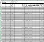
And my Helper Sheet
I have 2 Sheets. Output Sheet & Helper Sheet. I want to extract all the values that meets criteria from Helper Sheet, copy all that and paste it to the Output Sheet. And some more additional tasks if you could accommodate.
I would like to copy and paste all the cells from Helper Sheet Column D and Column F over to Output Sheet Column D and G respectively, if OutputSheet Cell D8 & D9 value is equal to the rows of Helper Sheet Column B & C.
After that, I would also like to copy down the formulas in OutputSheet to the last non blank rows of Column D. Notice I already have formulas set up in Cells B13, C13, F13, H13 & I13.
Then paste formulas from another sheet (A1:H4) in that newly created rows.
Here's my the output sheet.
| OTC-Sample-Sheet-v19.xlsm | ||||||||||||||
|---|---|---|---|---|---|---|---|---|---|---|---|---|---|---|
| A | B | C | D | E | F | G | H | I | J | K | L | |||
| 8 | Property, Plant and Equipment: | AMPLIFIER | ||||||||||||
| 9 | Object Account Code: | 1-06-05-070-001-000-000 | ||||||||||||
| 10 | Account Title: | Communication Equipment | ||||||||||||
| 11 | ||||||||||||||
| 12 | Date | Reference | PO-Contract Number | Description | Qty. | Unit Cost | Total Cost | Accumulated Depreciation | Accumulated Impairment Losses | Issues/ Transfers/ Adjustment/s | Adjusted Cost | |||
| 13 | #N/A | #N/A | 0 | 0.00 | 0.00 | 0.00 | ||||||||
| 14 | ||||||||||||||
| 15 | ||||||||||||||
| 16 | ||||||||||||||
| 17 | ||||||||||||||
| 18 | ||||||||||||||
| 19 | ||||||||||||||
| 20 | ||||||||||||||
| 21 | ||||||||||||||
| 22 | ||||||||||||||
| 23 | ||||||||||||||
| 24 | ||||||||||||||
| 25 | ||||||||||||||
| 26 | ||||||||||||||
| 27 | ||||||||||||||
| 28 | ||||||||||||||
| 29 | ||||||||||||||
| 30 | ||||||||||||||
| 31 | ||||||||||||||
| 32 | ||||||||||||||
| 33 | ||||||||||||||
| 34 | ||||||||||||||
| 35 | GRAND TOTAL | 0.00 | 0.00 | 0.00 | 0.00 | 0.00 | ||||||||
Output | ||||||||||||||
| Cell Formulas | ||
|---|---|---|
| Range | Formula | |
| D9 | D9 | =VLOOKUP(D8,CHOOSE({1,2},Helper!$B$1:$B$14,Helper!$C$1:$C$14),2,FALSE) |
| B13 | B13 | =VLOOKUP(C13,CHOOSE({1,2},JEV,Tdate),2,FALSE) |
| C13 | C13 | =VLOOKUP($D$8&$D$9&D13,CHOOSE({1,2},Table2[[#All],[Helper]],JEV),2,FALSE) |
| F13 | F13 | =COUNTIFS(TYPE,$D$8,ACCCODE,$D$9,PONUM,D13,COST,G13) |
| H13 | H13 | =+F13*G13 |
| I13 | I13 | =SUMIFS(BEGDEP,TYPE,$D$8,ACCCODE,$D$9,PONUM,D13,COST,G13) |
| L13 | L13 | =SUM(L12,H13:K13) |
| H35:K35 | H35 | =SUBTOTAL(9,H13:H34) |
| L35 | L35 | =SUM(H35:K35) |
| Press CTRL+SHIFT+ENTER to enter array formulas. | ||
| Named Ranges | ||
|---|---|---|
| Name | Refers To | Cells |
| Data!_FilterDatabase | =Data!$A$5:$P$70 | F13, I13 |
| ACCCODE | =Data!$B$5:$B$70 | F13, I13 |
| BEGDEP | =Data!$H$5:$H$70 | I13 |
| COST | =Data!$G$5:$G$70 | F13, I13 |
| JEV | =Data!$D$5:$D$70 | B13:C13 |
| PONUM | =Data!$C$5:$C$70 | F13, I13 |
| Tdate | =Data!$E$5:$E$70 | B13 |
| TYPE | =Data!$A$5:$A$70 | F13, I13 |
| Cells with Data Validation | ||
|---|---|---|
| Cell | Allow | Criteria |
| D8 | List | =Helper!$B$1:$B$14 |
And my Helper Sheet
| Cell Formulas | ||
|---|---|---|
| Range | Formula | |
| B4:C13 | B4 | =B3 |
| D12:D13,D9:D10,D5:D7 | D5 | =D4 |
| E2:E14 | E2 | =CONCATENATE(B2,C2,D2) |
| Press CTRL+SHIFT+ENTER to enter array formulas. | ||