Copying a column into another sheet from a reference point and up to a certain cell value

[kidneythief]

Hello! First off, apologies as I can't get my xl2bb add-in to work so I've attached images instead.

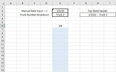
In the Output Sheet, there are two cells for inputs - one for the date (E2) and one for a truck number (E3).
Once these are filled in, they are combined into G3.

I need help with code that will take the contents of G3 as a reference and find its match in the Source Sheet.
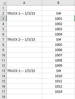
From there, I need to copy the numbers in the B2 column Source Sheet to the right of the G3 match, below the SI#
label up to the next SI# label.

So in the sample images, if G3 in the Output Sheet is "1/3/23--- Truck 2", I need to pull B8:B12 from Source Sheet and
copy them into the blue area in Output Sheet, below the SI# header.

My vba learning progress has been extremely slow Any help on this would be greatly appreciated!

 

[DanteAmor]

In your images, you have the date reversed.

But I'm going to assume that on both sheets, it should be like this:
TRUCK 2--- 1/3/23
Or whatever, but they are the same.

Try this:

Sub copytruck()
  Dim sh1 As Worksheet, sh2 As Worksheet
  Dim f As Range
  Dim truck As String
  Dim i As Long, j As Long
 
  Set sh1 = Sheets("Output")
  Set sh2 = Sheets("Source")
  truck = sh1.Range("G3").Value
 
  j = 7
  sh1.Range("E7:E" & Rows.Count).ClearContents
  If truck <> "" Then
    Set f = sh2.Range("A:A").Find(truck, , xlValues, xlWhole, , , False)
    If Not f Is Nothing Then
      For i = f.Row + 1 To sh2.Range("B" & Rows.Count).End(3).Row
        If sh2.Range("A" & i).Value <> "" Then
          Exit Sub
        Else
          sh1.Range("E" & j).Value = sh2.Range("B" & i).Value
          j = j + 1
        End If
      Next
    End If
  End If
End Sub

Or this:

Sub copytruck_2()
  Dim sh1 As Worksheet, sh2 As Worksheet
  Dim f As Range
  
  Set sh1 = Sheets("Output")
  Set sh2 = Sheets("Source")
  
  sh1.Range("E7:E" & Rows.Count).ClearContents
  If sh1.Range("G3").Value = "" Then Exit Sub
  Set f = sh2.Range("A:A").Find(sh1.Range("G3").Value, , xlValues, xlWhole, , , False)
  If Not f Is Nothing Then _
    f.Resize(sh2.Range("B" & Rows.Count).End(3).Row).SpecialCells(xlCellTypeBlanks).Areas(1).Offset(, 1).Copy sh1.Range("E7")
End Sub

 

[kidneythief]

Thank you Dante, the first one worked perfectly! I'm breaking down your code to try to learn from it and understand better, too. Also added a calculate sub to have the code run each time G3 changes.
Again, thanks for your time!