Count only one occurrence of all criteria being met

[ott3rpop]

I am trying to find a formula that will only count one or the first occurrence of when all the criteria I need are met.

I have a formula that will determine all instances that all criteria are met. Basically count how many times an employee appears in the list when the date is within this week, the status is complete, and the work done was a swap. This gives me the total jobs they completed this week.

=COUNTIFS(B:B,"*"&F2&"*",C:C,"SWAP",A:A,">="&TODAY()-WEEKDAY(TODAY(),3),A:A,"<"&TODAY()-WEEKDAY(TODAY(),3)+7,D:D,"COMPLETE")

I also want to find out how many days this week the employee appears in the list, with a complete status, and the work done was a swap. More than one job can be completed in a day, and more than one person can be assigned to a job.

My end goal is, I need to know how many days each employee worked so I can determine if they are working to full capacity for the week. For example, if an employee can complete 5 jobs a day and was scheduled for 5 days, they should have completed 25 jobs this week. Then I can compare that to how many they actually completed to determine if they are at, above, or below capacity. And eventually I want to do the same for YTD. So technically the "FIRST INSTANCE" column on my spreadsheet should be labeled "NUMBER OF DAYS WORKED".

The reason I need all the criteria to be met to determine how many days they worked, and not just the first time their name appears on a date is because if the status isn't complete, they may have been scheduled, but didn't work. And I need to track all this information as Swaps vs Cuts.

The first formula I am able to replace with a pivot table, but the issue I run into for tracking how many days a person worked is that more than one person is assigned to a job, and I don't know how to separate it by individual name, as a pivot table would only create 3 rows based on the current data.

Mark, Bob, Henry
Mark, Henry
Bob, Mark

But the rows I would need for a pivot table to work would be...

Mark
Bob
Henry

I also tried using a formula to separate the Employee column, so there is only one name per column, but I can't get that to work within a pivot table either. So the only thing I can think of is by doing it with a formula somehow, but I have tried lots of different formulas and can't figure out how to only count once per day this week count and employee if all other criteria are met.

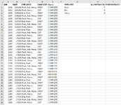
This is just a sample spreadsheet I made to get the basic info accross. The actual spreadsheet is updated daily with a report pulled from different software, so the info in columns A:E change every day as well.

If there is any other information I should have included or didn't explain well, please ask, I will answer anything I can.

 

[KRice]

Your description is confusing. You state that you want to count the first occurrence when all criteria are met (that would be a count of "one"...no counting is needed). Then you state that you have a formula that will determine all instances where all criteria are met. That's different.

Basically count how many times an employee appears in the list when the date is within this week, the status is complete, and the work done was a swap. This gives me the total jobs they completed this week.

...and then this:

I also want to find out how many days this week the employee appears in the list, with a complete status, and the work done was a swap. More than one job can be completed in a day, and more than one person can be assigned to a job.

Aren't both of these sentences saying the same thing?

So technically the "FIRST INSTANCE" column on my spreadsheet should be labeled "NUMBER OF DAYS WORKED".

This needs to be explained better. I am not sure about what you want, but I do understand the dilemma created by receiving data with employee names concatenated in a single field. You have suggested trying to split the names into separate columns, and I think that is a step in the right direction...especially if you have plans for more analysis of the data set. I would go further and unpivot the names to create a long, flat table that is well suited for counting operations. Normally, I would first consider using either Power Query or VBA to do the transformation, but you can achieve very similar results using formulas in Excel 365.

In the example below, I've left some intermediate results visible so that you can see what different parts of the formula do. The G2# formula splits out the names into a horizontal array for each row. The K2# formula takes the other data columns of interest--that are not to be unpivoted--and repeats them so that they will match up correctly with the names...after the names are stacked into a single column.

All of this is done in the P2# formula (so you don't need the G2 or K2 formulas...just delete them), which creates a flat table of your original data. I've also included an additional column for the week number associated with the Date. Using WEEKNUM is a more direct way of determining which entries occurred during the same week as TODAY(), so the "wn" (week number) array can be directly used in a counting formula. As for the counting formula, COUNTIF(S) will not accept an array name for the criteria range (as the name indicates, it must be a range reference, not an array), so I've shown an alternative approach using SUMPRODUCT. Depending on how long your flat table might become, the formula could become sluggish at very large sizes.

I do not know what you want for the "NUMBER OF DAYS WORKED" column. The data are in a more accessible format, but it's not clear what criteria should be applied. In the example below, I've truncated the worksheet snippet a few rows below your original table length due to size limitations. The formula in this example grows to three times the original length because there are three columns of employee names split out from the original data. What is the maximum number of names that might appear in the EMPLOYEE field on any given day? And approximately how many rows are your data tables as received?

MrExcel_20240229.xlsx
	A	B	C	D	E	F	G	H	I	J	K	L	M	N	O	P	Q	R	S	T	U	V	W	X	Y
1	JOB	DATE	EMPLOYEE	SWAP/CUT	Status											JOB	DATE	SWAP/CUT	Status	WEEKNUM	EMPLOYEE		EMPLOYEE	ALL INSTANCES	NUMBER OF DAYS WORKED
2	1234	2/25/2024	Mark, Bob, Henry	SWAP	COMPLETE		Mark	Bob	Henry		1234	45347	SWAP	COMPLETE		1234	45347	SWAP	COMPLETE	8	Mark		Mark	8
3	1235	2/25/2024	Mark, Henry	CUT	COMPLETE		Mark	Henry			1235	45347	CUT	COMPLETE		1235	45347	CUT	COMPLETE	8	Mark		Bob	5
4	1236	2/26/2024	Bob, Mark	SWAP	COMPLETE		Bob	Mark			1236	45348	SWAP	COMPLETE		1236	45348	SWAP	COMPLETE	9	Bob		Henry	5
5	1237	2/26/2024	Mark, Bob, Henry	SWAP	COMPLETE		Mark	Bob	Henry		1237	45348	SWAP	COMPLETE		1237	45348	SWAP	COMPLETE	9	Mark
6	1238	2/27/2024	Mark, Henry	CUT	COMPLETE		Mark	Henry			1238	45349	CUT	COMPLETE		1238	45349	CUT	COMPLETE	9	Mark
7	1239	2/27/2024	Bob, Mark	SWAP	COMPLETE		Bob	Mark			1239	45349	SWAP	COMPLETE		1239	45349	SWAP	COMPLETE	9	Bob
8	1240	2/28/2024	Mark, Bob, Henry	CUT	COMPLETE		Mark	Bob	Henry		1240	45350	CUT	COMPLETE		1240	45350	CUT	COMPLETE	9	Mark
9	1241	2/28/2024	Mark, Henry	SWAP	COMPLETE		Mark	Henry			1241	45350	SWAP	COMPLETE		1241	45350	SWAP	COMPLETE	9	Mark
10	1242	1/5/2024	Bob, Mark	SWAP	COMPLETE		Bob	Mark			1242	45296	SWAP	COMPLETE		1242	45296	SWAP	COMPLETE	1	Bob
11	1243	1/5/2024	Mark, Bob, Henry	CUT	COMPLETE		Mark	Bob	Henry		1243	45296	CUT	COMPLETE		1243	45296	CUT	COMPLETE	1	Mark
12	1244	1/6/2024	Mark, Henry	SWAP	COMPLETE		Mark	Henry			1244	45297	SWAP	COMPLETE		1244	45297	SWAP	COMPLETE	1	Mark
13	1245	1/6/2024	Bob, Mark	CUT	COMPLETE		Bob	Mark			1245	45297	CUT	COMPLETE		1245	45297	CUT	COMPLETE	1	Bob
14	1246	1/7/2024	Mark, Bob, Henry	SWAP	COMPLETE		Mark	Bob	Henry		1246	45298	SWAP	COMPLETE		1246	45298	SWAP	COMPLETE	1	Mark
15	1247	1/7/2024	Mark, Henry	SWAP	COMPLETE		Mark	Henry			1247	45298	SWAP	COMPLETE		1247	45298	SWAP	COMPLETE	1	Mark
16	1248	1/8/2024	Bob, Mark	CUT	COMPLETE		Bob	Mark			1248	45299	CUT	COMPLETE		1248	45299	CUT	COMPLETE	2	Bob
17	1249	1/8/2024	Mark, Bob, Henry	SWAP	COMPLETE		Mark	Bob	Henry		1249	45299	SWAP	COMPLETE		1249	45299	SWAP	COMPLETE	2	Mark
18	1250	1/9/2024	Mark, Henry	CUT	COMPLETE		Mark	Henry			1250	45300	CUT	COMPLETE		1250	45300	CUT	COMPLETE	2	Mark
19	1251	1/9/2024	Bob, Mark	SWAP	COMPLETE		Bob	Mark			1251	45300	SWAP	COMPLETE		1251	45300	SWAP	COMPLETE	2	Bob
20	1252	1/10/2024	Mark, Bob, Henry	SWAP	COMPLETE		Mark	Bob	Henry		1252	45301	SWAP	COMPLETE		1252	45301	SWAP	COMPLETE	2	Mark
21	1253	1/10/2024	Mark, Henry	CUT	COMPLETE		Mark	Henry			1253	45301	CUT	COMPLETE		1253	45301	CUT	COMPLETE	2	Mark
22	1254	2/25/2024	Bob, Mark	SWAP	COMPLETE		Bob	Mark			1254	45347	SWAP	COMPLETE		1254	45347	SWAP	COMPLETE	8	Bob
23	1255	2/25/2024	Mark, Bob, Henry	CUT	COMPLETE		Mark	Bob	Henry		1255	45347	CUT	COMPLETE		1255	45347	CUT	COMPLETE	8	Mark
24	1256	2/26/2024	Mark, Henry	SWAP	COMPLETE		Mark	Henry			1256	45348	SWAP	COMPLETE		1256	45348	SWAP	COMPLETE	9	Mark
25	1257	2/26/2024	Bob, Mark	SWAP	COMPLETE		Bob	Mark			1257	45348	SWAP	COMPLETE		1257	45348	SWAP	COMPLETE	9	Bob
26	1258	2/27/2024	Mark, Bob, Henry	CUT	COMPLETE		Mark	Bob	Henry		1258	45349	CUT	COMPLETE		1258	45349	CUT	COMPLETE	9	Mark
27	1259	2/27/2024	Mark, Henry	SWAP	COMPLETE		Mark	Henry			1259	45349	SWAP	COMPLETE		1259	45349	SWAP	COMPLETE	9	Mark
28	1260	2/28/2024	Bob, Mark	CUT	COMPLETE		Bob	Mark			1260	45350	CUT	COMPLETE		1260	45350	CUT	COMPLETE	9	Bob
29	1261	2/28/2024	Mark, Bob, Henry	SWAP	COMPLETE		Mark	Bob	Henry		1261	45350	SWAP	COMPLETE		1261	45350	SWAP	COMPLETE	9	Mark
30	1262	1/5/2024	Mark, Henry	SWAP	COMPLETE		Mark	Henry			1262	45296	SWAP	COMPLETE		1262	45296	SWAP	COMPLETE	1	Mark
31	1263	1/5/2024	Bob, Mark	CUT	COMPLETE		Bob	Mark			1263	45296	CUT	COMPLETE		1263	45296	CUT	COMPLETE	1	Bob
32	1264	1/6/2024	Mark, Bob, Henry	SWAP	COMPLETE		Mark	Bob	Henry		1264	45297	SWAP	COMPLETE		1264	45297	SWAP	COMPLETE	1	Mark
33	1265	1/6/2024	Mark, Henry	CUT	COMPLETE		Mark	Henry			1265	45297	CUT	COMPLETE		1265	45297	CUT	COMPLETE	1	Mark
34	1266	1/7/2024	Bob, Mark	SWAP	COMPLETE		Bob	Mark			1266	45298	SWAP	COMPLETE		1266	45298	SWAP	COMPLETE	1	Bob
35	1267	1/7/2024	Mark, Bob, Henry	SWAP	COMPLETE		Mark	Bob	Henry		1267	45298	SWAP	COMPLETE		1267	45298	SWAP	COMPLETE	1	Mark
36	1258	1/8/2024	Mark, Henry	CUT	COMPLETE		Mark	Henry			1258	45299	CUT	COMPLETE		1258	45299	CUT	COMPLETE	2	Mark
37											1234	45347	SWAP	COMPLETE		1234	45347	SWAP	COMPLETE	8	Bob
38											1235	45347	CUT	COMPLETE		1235	45347	CUT	COMPLETE	8	Henry
39											1236	45348	SWAP	COMPLETE		1236	45348	SWAP	COMPLETE	9	Mark
40											1237	45348	SWAP	COMPLETE		1237	45348	SWAP	COMPLETE	9	Bob
41											1238	45349	CUT	COMPLETE		1238	45349	CUT	COMPLETE	9	Henry
Sheet1

Cell Formulas
Range	Formula
G2:I36	G2	=DROP(IFERROR(REDUCE(0,$C$2:$C$36,LAMBDA(a,b,VSTACK(a,TEXTSPLIT(b,", ")))),""),1)
K2:N106	K2	=LET(nemp,COLUMNS(G2#),data,CHOOSECOLS($A$2:$E$36,1,2,4,5),rdata,ROWS(data),res,REDUCE(data,SEQUENCE(nemp-1),LAMBDA(a,b,VSTACK(a,data))),res)
P2:U106	P2	=LET(source,$A:$E, lrow,MATCH(1E+100,$A:$A), data, DROP(TAKE(source,lrow),1), emp, DROP(IFERROR(REDUCE(0,CHOOSECOLS(data,3),LAMBDA(a,b,VSTACK(a,TEXTSPLIT(b,", ")))),""),1), nemp,COLUMNS(emp), nndata,HSTACK(CHOOSECOLS(data,1,2,4,5),WEEKNUM(CHOOSECOLS(data,2),2)),rdata,ROWS(data),nndata_stacked,REDUCE(nndata,SEQUENCE(nemp-1),LAMBDA(a,b,VSTACK(a,nndata))),HSTACK(nndata_stacked,TOCOL(emp,,TRUE)))
W2:W4	W2	=UNIQUE(TOCOL(DROP(REDUCE(0,$C$2:$C$36,LAMBDA(a,b,VSTACK(a,TEXTSPLIT(b,", ")))),1),3))
X2:X4	X2	=LET(data,$P$2#,sc,CHOOSECOLS(data,3),st,CHOOSECOLS(data,4),wn,CHOOSECOLS(data,5),emp, CHOOSECOLS(data,6), resALL, SUMPRODUCT( (wn=WEEKNUM(TODAY(),2)) * (emp=W2) * (sc="SWAP") * (st="COMPLETE") ), resALL)
Dynamic array formulas.

 

[ott3rpop]

Your description is confusing. You state that you want to count the first occurrence when all criteria are met (that would be a count of "one"...no counting is needed). Then you state that you have a formula that will determine all instances where all criteria are met. That's diff

Yes, the formula I have is different from what I am asking for help with. I also need this formula. I need to know both sets of information; all instances that criteria are met within a week per employee and how many days this week all criteria are met per employee. I included this to show what I have so far incase it can be altered to accomplish the second parameters.

Aren't both of these sentences saying the same thing?

They aren't the same. The first thing I need, and the formula I do have, tells me all completed jobs in a week per employee, that number could be anywhere from zero to 30+. I also need to know how many days this week an employee completed a job, that number can't be higher than 5 (working M-F, a total of 5 days potentially).

This needs to be explained better. I am not sure about what you want

My end goal is to determine how many days this week an employee worked. So if I can count only the first instance per day this week that all criteria are met, that would get me the number of days they worked. That's what I don't know how to do, I don't know how to only count one instance per day. I've only been able to figure out how to count all instances within a week.

You have suggested trying to split the names into separate columns, and I think that is a step in the right direction

I tried this, but I still couldn't figure out a formula to only count the first (or one) instance per day.

I also want to avoid adding a significant amount of new columns with formulas to my spreadsheet. The actual spreadsheet is very large, adding a lot more to it causes it to be bogged down and unusable unfortunately. I could potentially add a column to calculate the week number. Would that change my formula from this...

=COUNTIFS(B:B,"*"&F2&"*",C:C,"SWAP",A:A,">="&TODAY()-WEEKDAY(TODAY(),3),A:A,"<"&TODAY()-WEEKDAY(TODAY(),3)+7,D:D,"COMPLETE")

to...
=COUNTIFS(B:B,"*"&F2&"*",C:C,"SWAP",F:F,=WEEKNUM(TODAY()),D:D,"COMPLETE")

Assuming F:F would be my new column with the week number?

 

[KRice]

Thanks for the clarification...I think I understand now. So the distinction is that one is a count of the number of jobs during the week, the other is a count of the number of days during the week...and both counts require other criteria to be satisfied. Regarding your comment about adding new columns, what I posted was intended only to show what the formula is doing internally...it creates an internal array that can be used to deliver the results needed without displaying anything other than the results...no additional columns would be needed. Below is an example where the formulas presented have been consolidated and slightly revised to deliver what you want.

I'll attempt to step through the formula to describe the various parts: The source data is defined with whole column references, which seems to be your preference. Next, the last row (lrow) of the source data is determined using column A. Then a multi-column array called "data" is defined by trimming down the size of the "source" so that it includes only the rows where data are found. Assuming the employee names are found in column 3 of "source", we split apart multiple names in the Employee Names column using a comma space ", " as the delimiter. This creates a two-dimensional array with names appearing across the columns for each row. The number of columns of this two-dimensional array is determined ("nemp"). Because so much of the analysis depends on knowing if something occurred during the same week, it is convenient to know the week number, so an array of week numbers associated with each date in "data" is created and appended (horizontally) to columns 1,2,4, and 5 of data (Job, Date, Swap/Cut, and Status), and this array is called "nndata" to reflect that it is based on the original "data" but no names are included. This "nndata" array needs to be stacked onto itself multiple times and then aligned with the unpivoted names. To do this, a new variable called "nndata_stacked" is defined using a LAMBDA function to repeatedly stack "nndata" based on the number of columns in the split-names array ("nemp"). Finally, this vertically stacked array is combined (horizontally) with the employee names that were previously split apart...all of those names are stacked vertically, column-by-column to align correctly with "nndata_stacked". This new array is "flat" and very convenient for subsequent use in determining the quantities of interest. The new data array is called "fdata" to indicate is it flat.

For convenience, the various columns of "fdata" are assigned to more meaningful variable names: "dt" for dates, "sc" for swap/cut, "st" for status, "wn" for week number, and "emp" for employee name. Then the counts desired are given using a FILTER function to extract all of the date ("dt") entries where the criterial are met. Where a total number of assignments is desired, the number of dates is counted ("resAll" for results All). Where the total number of days is desired, the UNIQUE function is used to include only unique dates, and those are counted ("resNdays" for results Number of days). Both results are stacked horizontally and delivered as one array.

MrExcel_20240229.xlsx
	A	B	C	D	E	F	G	H	I
1	JOB	DATE	EMPLOYEE	SWAP/CUT	Status		EMPLOYEE	ALL INSTANCES	NUMBER OF DAYS WORKED
2	1234	2/25/2024	Mark, Bob, Henry	SWAP	COMPLETE		Mark	8	3
3	1235	2/25/2024	Mark, Henry	CUT	COMPLETE		Bob	5	3
4	1236	2/26/2024	Bob, Mark	SWAP	COMPLETE		Henry	5	3
5	1237	2/26/2024	Mark, Bob, Henry	SWAP	COMPLETE
6	1238	2/27/2024	Mark, Henry	CUT	COMPLETE
7	1239	2/27/2024	Bob, Mark	SWAP	COMPLETE
8	1240	2/28/2024	Mark, Bob, Henry	CUT	COMPLETE
9	1241	2/28/2024	Mark, Henry	SWAP	COMPLETE
10	1242	1/5/2024	Bob, Mark	SWAP	COMPLETE
11	1243	1/5/2024	Mark, Bob, Henry	CUT	COMPLETE
12	1244	1/6/2024	Mark, Henry	SWAP	COMPLETE
13	1245	1/6/2024	Bob, Mark	CUT	COMPLETE
14	1246	1/7/2024	Mark, Bob, Henry	SWAP	COMPLETE
15	1247	1/7/2024	Mark, Henry	SWAP	COMPLETE
16	1248	1/8/2024	Bob, Mark	CUT	COMPLETE
17	1249	1/8/2024	Mark, Bob, Henry	SWAP	COMPLETE
18	1250	1/9/2024	Mark, Henry	CUT	COMPLETE
19	1251	1/9/2024	Bob, Mark	SWAP	COMPLETE
20	1252	1/10/2024	Mark, Bob, Henry	SWAP	COMPLETE
21	1253	1/10/2024	Mark, Henry	CUT	COMPLETE
22	1254	2/25/2024	Bob, Mark	SWAP	COMPLETE
23	1255	2/25/2024	Mark, Bob, Henry	CUT	COMPLETE
24	1256	2/26/2024	Mark, Henry	SWAP	COMPLETE
25	1257	2/26/2024	Bob, Mark	SWAP	COMPLETE
26	1258	2/27/2024	Mark, Bob, Henry	CUT	COMPLETE
27	1259	2/27/2024	Mark, Henry	SWAP	COMPLETE
28	1260	2/28/2024	Bob, Mark	CUT	COMPLETE
29	1261	2/28/2024	Mark, Bob, Henry	SWAP	COMPLETE
30	1262	1/5/2024	Mark, Henry	SWAP	COMPLETE
31	1263	1/5/2024	Bob, Mark	CUT	COMPLETE
32	1264	1/6/2024	Mark, Bob, Henry	SWAP	COMPLETE
33	1265	1/6/2024	Mark, Henry	CUT	COMPLETE
34	1266	1/7/2024	Bob, Mark	SWAP	COMPLETE
35	1267	1/7/2024	Mark, Bob, Henry	SWAP	COMPLETE
36	1258	1/8/2024	Mark, Henry	CUT	COMPLETE
Sheet1

Cell Formulas
Range	Formula
G2:G4	G2	=LET(source,$C:$C, lrow,MATCH(1E+100,$A:$A), data,DROP(TAKE(source,lrow),1),UNIQUE(TOCOL(DROP(REDUCE(0,data,LAMBDA(a,b,VSTACK(a,TEXTSPLIT(b,", ")))),1),3)) )
H2:I4	H2	=LET(source,$A:$E, lrow,MATCH(1E+100,$A:$A), data,DROP(TAKE(source,lrow),1), empsrc, DROP(IFERROR(REDUCE(0,CHOOSECOLS(data,3),LAMBDA(a,b,VSTACK(a,TEXTSPLIT(b,", ")))),""),1), nemp,COLUMNS(empsrc), nndata,HSTACK(CHOOSECOLS(data,1,2,4,5),WEEKNUM(CHOOSECOLS(data,2),2)), nndata_stacked,REDUCE(nndata,SEQUENCE(nemp-1),LAMBDA(a,b,VSTACK(a,nndata))), fdata, HSTACK(nndata_stacked,TOCOL(empsrc,,TRUE)), dt,CHOOSECOLS(fdata,2), sc,CHOOSECOLS(fdata,3), st,CHOOSECOLS(fdata,4), wn,CHOOSECOLS(fdata,5), emp, CHOOSECOLS(fdata,6), resALL, COUNTA(FILTER(dt,(wn=WEEKNUM(TODAY(),2)) * (emp=G2) * (sc="SWAP") * (st="COMPLETE") )), resNdays, COUNTA(UNIQUE(FILTER(dt,(wn=WEEKNUM(TODAY(),2)) * (emp=G2) * (sc="SWAP") * (st="COMPLETE") ))), HSTACK(resALL,resNdays))
Dynamic array formulas.

 

[ott3rpop]

I finally had time today to work on this. Your formulas are so far out of my excel abilities I am not even sure I understand your explanations! This is WAY more advanced than I am currently capable of. That being said, I would love to try it out with my spreadsheet and see if I can get it to work!

=LET(source,$C:$C, lrow,MATCH(1E+100,$A:$A), data,DROP(TAKE(source,lrow),1),UNIQUE(TOCOL(DROP(REDUCE(0,data,LAMBDA(a,b,VSTACK(a,TEXTSPLIT(b,", ")))),1),3)) )

Do I need to change anything within this formula other than $C:$C and $A:$A to customize it to fit my actual spreadsheet? Or are there other variables within the formula that I need to change to match my data set? In my spreadsheet $C:$C would be $CX:$CX. And $A:$A would be $B:$B.

Once I get this part of it working for me I will ask how to customize the second formula. Baby steps since this is so far out of my wheelhouse.

 

[KRice]

Yes...your plans for adapting the formula sound correct. This formula does nothing more than create a list of employees. If you'd like, that list could also appear sorted (the formula doesn't do that as written, but adding that step would be easy). The only "hooks" into your sheet are those two column specifications. Column C/CX would list the names, perhaps in some cases separated by a "comma space". You'll see that delimiter in the formula near the end. If a different delimiter is used in your actual file, or if the delimiter is a comma and no space, or a comma and two spaces, then either some data clean up might be needed to make everything consistent, or change the delimiter in the formula. Regarding the column A/(or B in your latest case), the formula is assuming that column contains numbers, not text. The idea is that we use the MATCH function to look down the column for a ridiculously large number that doesn't actually exist in the column, and MATCH will return the last row number...and that is used to limit the size of the data array used in the formula without having to hardwire in the actual data range.

Once you have that working, post back...an additional adjustment might be needed on the other formula, as the current one assumes you'll be specifying 5 adjacent columns, and it sounds as if that may not be the case...easily fixed, but will need some details.

 

[ott3rpop]

Regarding the column A/(or B in your latest case), the formula is assuming that column contains numbers, not text.

My actual job numbers contain both letters and numbers, for example: L12B4C0- Swap (C22) or KB-422-A01-L2 (Swap) B40

I have no control over this, I think they auto-generated by the software. Sorry, I didn't realize the formula depended on the job numbers being only numbers. Is there a way to change to formula to make it work with non-number data?

 

[KRice]

Yes, sure is…I’ll post back when I get to a computer.

 

[KRice]

If there is nothing below the "A" column, which I think you said would be your "B" column...we could change up the way the last row number is found by using this revised "lrow" formula (see lrow on the first line). This type of formula evaluates whether the A column cells are not blank. Blank cells will evaluate as FALSE (A<>""), while cells with something in them (text or number...doesn't matter) will evaluate as TRUE. We divide the array of TRUE/FALSE into 1, which coerces TRUEs to 1's and FALSE;s to 0's...and the array will consist of 1's and #DIV/0! errors. LOOKUP then searches this array for the number 2 (which doesn't exist), so it's default behavior is to find the last non-error position, and we return the ROW number for that position. We don't have to use column A (or B) for this last row determination...any column will work, provided it's last cell corresponding to the bottom of the table contains data.

=LET(source,$A:$E, lrow,LOOKUP(2,1/($A:$A<>""),ROW($A:$A)),
data,DROP(TAKE(source,lrow),1),
empsrc, DROP(IFERROR(REDUCE(0,CHOOSECOLS(data,3),LAMBDA(a,b,VSTACK(a,TEXTSPLIT(b,", ")))),""),1),
nemp,COLUMNS(empsrc),
nndata,HSTACK(CHOOSECOLS(data,1,2,4,5),WEEKNUM(CHOOSECOLS(data,2),2)),
nndata_stacked,REDUCE(nndata,SEQUENCE(nemp-1),LAMBDA(a,b,VSTACK(a,nndata))),
fdata, HSTACK(nndata_stacked,TOCOL(empsrc,,TRUE)),
dt,CHOOSECOLS(fdata,2),  sc,CHOOSECOLS(fdata,3),  st,CHOOSECOLS(fdata,4),  wn,CHOOSECOLS(fdata,5),  emp, CHOOSECOLS(fdata,6),
resALL,      COUNTA(FILTER(dt,(wn=WEEKNUM(TODAY(),2)) * (emp=G2) * (sc="SWAP") * (st="COMPLETE") )),
resNdays, COUNTA(UNIQUE(FILTER(dt,(wn=WEEKNUM(TODAY(),2)) * (emp=G2) * (sc="SWAP") * (st="COMPLETE") ))),
HSTACK(resALL,resNdays))