Count unique values with sum-frequency array? multiple countifs? or other formulas?

[dexiw]

Hi everyone,

Sorry if I am overlooking other resources on this forum regarding a similar question.

I am currently using a sum-frequency array formula to calculate how many unique police precincts:
1) have operational interventions in a given year; and
2) see a decrease in burglaries from one year to the next.

Please note the following about the police precincts:
1) it is possible that there could be smaller intervention sites in a police precinct, which could have operational or inoperable interventions at the end of each year; and
2) the # of burglaries might only be reported at the level of a police precinct (which you can think of as the largest police jurisdiction type). This means that smaller intervention sites, in certain cases, won't have any burglary data because the police force can only report for all intervention sites at the level of a police precinct.

The array formula that I have drafted thus far is counting the unique police precincts per year correctly (when that is the only criteria in the formula)... but not the # of unique precincts that see a decrease in burglaries from one year to the next. Instead, the array formula seems to look at the # of burglaries in precincts with interventions for a given year, aggregates the # of burglaries for that year, and then compares that result to the # of burglaries for the next year. However, this does provide the correct result.

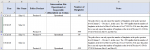
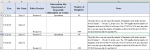
I have pasted what the raw data looks like for two police precincts below.

This is the raw data, for Precinct #1:

This is the raw data, for Precinct #2:

I am pasting different versions of the array formulas (which are more or less the same from one another) below. The arrays formula looks at all the raw data provided above in order to calculate the result. The word "DCT" in each array formula below is just the name of the tab (which I'm sure that you already knew/could have surmised).

Array #1:
=SUM(--(FREQUENCY(IF((DCT!$C$2:$C$9997<>"")*(DCT!$A$2:$A$9997="CY2016")*(DCT!$E$2:$E$9997="Operational")*(DCT!$F$2:$F$9997>=0)*(DCT!$F$2:$F$9997<>"")*(SUMIFS(DCT!$F$2:$F$9997,DCT!$A$2:$A$9997,"CY2015",DCT!$E$2:$E$9997,"Operational",DCT!$F$2:$F$9997,">=0")>SUMIFS(DCT!$F$2:$F$9997,DCT!$A$2:$A$9997,"CY2016",DCT!$E$2:$E$9997,"Operational",DCT!$F$2:$F$9997,">=0")),MATCH(DCT!$C$2:$C$9997,DCT!$C$2:$C$9997,0)),ROW(DCT!$C$2:$C$9997)-ROW(DCT!$C$2)+1)>0))
Result from Array #1 for CY2016 = 2

Array #3:
=SUM(--(FREQUENCY(IF((DCT!$C$2:$C$9997<>"")*(DCT!$A$2:$A$9997="CY2016")*(DCT!$E$2:$E$9997="Operational")*(DCT!$F$2:$F$9997>=0)*(DCT!$F$2:$F$9997<>"")*(IF(SUMIFS(DCT!$F$2:$F$9997,DCT!$A$2:$A$9997,"CY2015",DCT!$E$2:$E$9997,"Operational",DCT!$F$2:$F$9997,">=0")>SUMIFS(DCT!$F$2:$F$9997,DCT!$A$2:$A$9997,"CY2016",DCT!$E$2:$E$9997,"Operational",DCT!$F$2:$F$9997,">=0"),"1","0")),MATCH(DCT!$C$2:$C$9997,DCT!$C$2:$C$9997,0)),ROW(DCT!$C$2:$C$9997)-ROW(DCT!$C$2)+1)>0))
Result from Array #2 for CY2016 = 2

The CY2016 result for each array formula, based on the raw data, should be 1, not 2. This is because Precinct #2 saw its burglaries decrease from CY2015 to CY2016, whereas Precinct #1 saw its burglaries increase in the same time period.

If it is not possible to have just *one* formula that calculates the result, that's fine. Similarly, if what I need to use is a completely different formula type, please direct me in the right direction.

Thanks!

 

[J.Ty.]

Do you always want to compare directly two years?

J.Ty.

 

[dexiw]

For the moment, yes, just two years (sequential) compared to one another. There is a possibility down the road that non-sequential years might be compared, but we'll cross that bridge when we get to it.

Let me know if you need anything else, J.Ty.

 

[J.Ty.]

I need to reconstruct my understanding back then
Seriously, when I watch my formulas after a month, I feel like they were written by somebody else, who understands much more than I do. But I will manage it, it will only take a while.

J.Ty.

 

[dexiw]

Totally fair! I had the same issue when I finally had time to come back to this chain.

Appreciate your time and support!

 

[J.Ty.]

Juest to make it sure: are the results for 2015 and 2016 correct?

 

[dexiw]

It doesn't matter which years you use in your example. I'll update accordingly per formula. 2015 and 2016 are fine in your example though.

 

[J.Ty.]

I meant something different. If you get the same results no matter which years you compare, then the question arises if you can trust the results that seemed correct at first.

However:
I did experiments on small sample of artificial data and the results differ, if the underlying data changes.

Book1
	A	B	C	D
1	Precinct #2	1	Yes	Yes
2	Precinct #2	2
3	Precinct #1	1	No	Yes
4	Precinct #1	2
5	Precinct #2	3
6	Precinct #1	3
7	Precinct #2	4
8	Precinct #1	4
Sheet2

Cell Formulas
Range	Formula
B1:B8	B1	=COUNTIF($A$1:$A1,A1)
C1:C8	C1	=IF(B1=1,IF(SUMIFS(DCT!$F$3:$F$12,DCT!$A$3:$A$12,"CY2015",DCT!$E$3:$E$12,"Operational",DCT!$C$3:$C$12,A1)>SUMIFS(DCT!$F$3:$F$12,DCT!$A$3:$A$12,"CY2016",DCT!$E$3:$E$12,"Operational",DCT!$C$3:$C$12,A1),"Yes","No"),"")
D1:D8	D1	=IF(B1=1,IF(SUMIFS(DCT!$F$3:$F$12,DCT!$A$3:$A$12,"CY2016",DCT!$E$3:$E$12,"Operational",DCT!$C$3:$C$12,A1)>SUMIFS(DCT!$F$3:$F$12,DCT!$A$3:$A$12,"CY2017",DCT!$E$3:$E$12,"Operational",DCT!$C$3:$C$12,A1),"Yes","No"),"")

Now let us compare the two formulas:

=IF(B1=1,IF(SUMIFS(DCT!$F$3:$F$12,DCT!$A$3:$A$12,"CY2015",DCT!$E$3:$E$12,"Operational",DCT!$C$3:$C$12,A1)>SUMIFS(DCT!$F$3:$F$12,DCT!$A$3:$A$12,"CY2016",DCT!$E$3:$E$12,"Operational",DCT!$C$3:$C$12,A1),"Yes","No"),"")

=IF(B1=1,IF(SUMIFS(DCT!$F$3:$F$12,DCT!$A$3:$A$12,"CY2016",DCT!$E$3:$E$12,"Operational",DCT!$C$3:$C$12,A1)>SUMIFS(DCT!$F$3:$F$12,DCT!$A$3:$A$12,"CY2017",DCT!$E$3:$E$12,"Operational",DCT!$C$3:$C$12,A1),"Yes","No"),"")

The green parameters should have changed and did.
However, the red parameters are identical, but do not have $ in front of column names. It means that if you copy the first formula to the next column, A1 will become B1, which is something completely different. I had to change them manually to get the second formula, because I had not designed those formulas to be copied horizontally.

Might that be the reason?

J.Ty.

 

[dexiw]

Hi J.Ty.

That seemed to work. Not sure what the issue was before.

The more that I think about it, I also want to ensure that any negative or possible text responses in Column F are excluded. When I included additional criteria to each SUMIFS statement, the formula did not work like I expected. For example, after A1 in each SUMIFs statement, I added:
1. ,DCT!$F$3:$F$12,">-1"
2. ,DCT!$F$3:$F$12 ,"<>N/A"

But, the result from adding those two additional criteria was the incorrect result.

Do you have any suggestions for how to exclude negative responses and possible text entries in Column F? While I understand that I can make the column restricted to numeric fields, my team has rejected my proposal (for the time being) and wants users to be able to enter N/A or N/C when data is not applicable or not collectible, for example.

Thanks again.

 

[J.Ty.]

Hi J.Ty.

That seemed to work. Not sure what the issue was before.

The more that I think about it, I also want to ensure that any negative or possible text responses in Column F are excluded. When I included additional criteria to each SUMIFS statement, the formula did not work like I expected. For example, after A1 in each SUMIFs statement, I added:
1. ,DCT!$F$3:$F$12,">-1"
2. ,DCT!$F$3:$F$12 ,"<>N/A"

But, the result from adding those two additional criteria was the incorrect result.

Do you have any suggestions for how to exclude negative responses and possible text entries in Column F? While I understand that I can make the column restricted to numeric fields, my team has rejected my proposal (for the time being) and wants users to be able to enter N/A or N/C when data is not applicable or not collectible, for example.

Thanks again.

Use
=IF(B1=1,IF(SUMPRODUCT(DCT!$F$3:$F$12,DCT!$F$3:$F$12,">-1",DCT!$A$3:$A$12,"CY2015",DCT!$E$3:$E$12,"Operational",DCT!$C$3:$C$12,A1)> SUMIFS(DCT!$F$3:$F$12,DCT!$F$3:$F$12,">-1",DCT!$A$3:$A$12,"CY2016",DCT!$E$3:$E$12,"Operational",DCT!$C$3:$C$12,A1),"Yes","No"),"")

The filter ">-1" in SUMIFS excludes texts and error values, too. You can test in on a simpler example, like the one below:

Book1
	H	I
8	1	#N/A
9	2	5
10	#N/A	#N/A
11	2
12	Allan
Sheet5

Cell Formulas
Range	Formula
I8	I8	=SUM(H8:H12)
I9	I9	=SUMIFS(H8:H12,H8:H12,">-1")
H10	H10	=NA()
I10	I10	=SUMIFS(H8:H12,H8:H12,"<>"&NA())

 

[dexiw]

Hi J.Ty.

Thanks for this.

Confirming whether the first part of the formula should be SUMPRODUCT rather than SUMIFS? If so, I get an error value.

When changing the SUMPRODUCT to SUMIFS, I find that the formula works in some instances and not in others. For example, in my version of your Column I above, the formula didn't work. However, when I created a new column for 2016 and 2017 data, the formula did work. I'm still trying to sort out why that would be on my end.

Any thoughts that you might have about the above two points would be appreciated.