Countif contra formula

[kingjet]

Hi All,



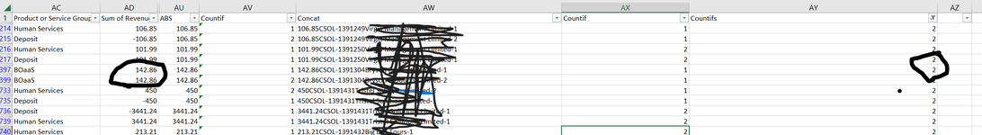
I thought this formula was working as it did find a lot of contra entries, which then shown in column AJ a 1 or 2 – 2 meant it has a matching contra based on the concat in AI, 1 meant it cannot find a matching entry



I was happy until I randomly checked an amount (180) and realised it as 1 when it should have been 2



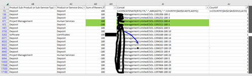
In column AD it counts how many 180 there are above (its filtered on 180) - its got over 100,000 lines so if you look at cell AI 971, at the end it says 180-4, this is because it looks at column AD and see how many times before 180 has come - so it says its seen 180- 4 times before ( i am trying to net the same figures) problem is row 973 should match 971 but BECAUSE the concat at the end says 180-4 & 180-1 it counts that as two separate lines (non matching) and gives me the incorrect number 1 in column AJ


if you look at column AI cells 971 and 973 they are exactly the same and should net off, but due to concat and countifs it doesn’t match, it thinks its different

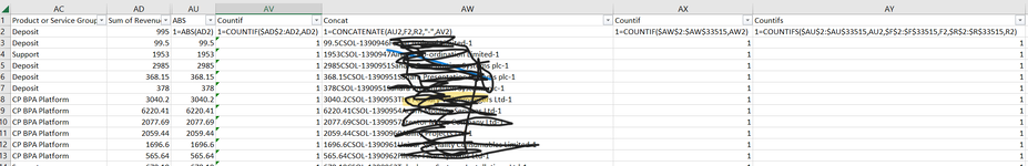
I also I think need the countifs formula in Column AI as it if do not the countif in column AJ will show more numbers than 1 or 2 which is incorrect



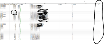
As an exercise I deleted the 180’s in cells AD 73,136,220 and guess what the cell AJ 971/972 show a 2


btw the concat is the invoice number, client name, and the amount - to make it very unique

 

[kingjet]

Hello picture 1 shows my same formulas : where your D2:J2 mine is AU2:AY2 - ive purposely shown you the formulas

picture 2 - shows that there are two 142 amounts and they should not be 2 in column AY

picture 3 shows - many numbers in AY- i was expecting 2 for all matching and 1 for no matching - but i have 1,2,3,4,15,16,17,18 etc

 

[kingjet]

sorry in your formula for J2 you are doing from D2 to D39 but in G2 go all the way down to 33515. in my formula in j2 i go down to 33515 too?

 

[kingjet]

i have tried imiating my file for you

XL22XB test.xlsx
	A	B	C	D	E	F	G	H
1	Invoice Number		Sum of Revenue	ABS	Countif	Concat	Countif	Countifs
2	CSOL-1390946		995	995	1	995CSOL-1390946-1	2	3
3	CSOL-1390946		99.5	99.5	1	99.5CSOL-1390946-1	1	1
4	CSOL-1390947		1953	1953	1	1953CSOL-1390947-1	1	1
5	CSOL-1390946		-995	995	1	995CSOL-1390946-1	2	3
6	CSOL-1390946		-995	995	2	995CSOL-1390946-2	1	3
7	CSOL-1390951		368.15	368.15	1	368.15CSOL-1390951-1	1	1
8	CSOL-1390951		378	378	1	378CSOL-1390951-1	1	1
9	CSOL-1390953		3040.2	3040.2	1	3040.2CSOL-1390953-1	1	1
10	CSOL-1390954		6220.41	6220.41	1	6220.41CSOL-1390954-1	1	1
11	CSOL-1390957		2077.69	2077.69	1	2077.69CSOL-1390957-1	1	1
12	CSOL-1390960		2059.44	2059.44	1	2059.44CSOL-1390960-1	1	1
13	CSOL-1390961		1696.6	1696.6	1	1696.6CSOL-1390961-1	1	1
14	CSOL-1390962		565.64	565.64	1	565.64CSOL-1390962-1	1	1
15	CSOL-1390963		678.19	678.19	1	678.19CSOL-1390963-1	1	1
16	CSOL-1390963		3049.36	3049.36	1	3049.36CSOL-1390963-1	1	1
17	CSOL-1390964		884.34	884.34	1	884.34CSOL-1390964-1	1	1
18	CSOL-1390964		1244.82	1244.82	1	1244.82CSOL-1390964-1	1	1
19	CSOL-1390964		548.2	548.2	1	548.2CSOL-1390964-1	1	1
20	CSOL-1390964		4594.64	4594.64	1	4594.64CSOL-1390964-1	1	1
21	CSOL-1391075		180	180	1	180CSOL-1391075-1	1	1
22	CSOL-1391208		180	180	2	180CSOL-1391208-2	1	1
23	CSOL-1391252		180	180	3	180CSOL-1391252-3	1	1
24	CSOL-1391511		180	180	4	180CSOL-1391511-4	1	2
25	CSOL-1391511		-180	180	1	180CSOL-1391511-1	1	2
26	CSOL-1391304		142.86	142.86	1	142.86CSOL-1391304-1	1	2
27	CSOL-1391304		142.86	142.86	2	142.86CSOL-1391304-2	1	2
28	CSOL-1393201		142.86	142.86	5	142.86CSOL-1393201-5	1	2
29	CSOL-1393201		142.86	142.86	6	142.86CSOL-1393201-6	1	2
30	CSOL-1394959		142.86	142.86	10	142.86CSOL-1394959-10	1	2
31	CSOL-1394959		142.86	142.86	11	142.86CSOL-1394959-11	1	2
32	CSOL-1396996		142.86	142.86	15	142.86CSOL-1396996-15	1	2
33	CSOL-1396996		142.86	142.86	16	142.86CSOL-1396996-16	1	2
34	CSOL-1399024		142.86	142.86	18	142.86CSOL-1399024-18	1	2
35	CSOL-1399024		142.86	142.86	19	142.86CSOL-1399024-19	1	2
36	CSOL-1401451		142.86	142.86	22	142.86CSOL-1401451-22	1	2
37	CSOL-1401451		142.86	142.86	23	142.86CSOL-1401451-23	1	2
38
39								also in this column in the original file I have more than 2 - so I have 1,2,4,5,6,7,8 - I really want to see 2 and 1
Sheet1

Cell Formulas
Range	Formula
D2:D20	D2	=ABS(C2)
E2:E20	E2	=COUNTIF($C$2:C2,C2)
F2:F20	F2	=CONCATENATE(D2,A2,B2,"-",E2)
G2:G25	G2	=COUNTIF($F$2:$F$33516,F2)
H2:H25	H2	=COUNTIFS($D$2:$D$33516,D2,$A$2:$A$33516,A2)

 

[jorismoerings]

Hi,


If you have a result of 4 and only expecting a result of max 2, this would mean the combination of invoice number, client name, and the amount isn't unique in your file while it is in the sample file. You'll need to find a better concat combination to identy the 2 lines belonging together. I can't help you with your data in the example isn't matching with the file you need it for.