COUNTIF on different sheet and across a range of cells

[Griff687]

Hi everyone,
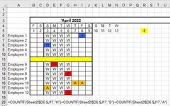
I have an attendance sheet that I want to count the number of cumulative days employees are off work, either on Holiday, Sick or Absent for any other reason.
The way the sheet denotes this is by entering either "H", "S" or "A" into the cell representing that day.
I've tried a number of COUNTIF's but none of them are giving me what I want - here's the latest attempt (notice that it refers to a range because I want info for the whole week):
{=COUNTIF('Sheet1'!$L49:$ML74,"=H")+COUNTIF('Sheet1'!$L49:$ML74,"=S")+COUNTIF('Sheet1'!$L49:$ML74,"=A")}
I've entered it as a normal formula and an Array (Ctrl+Shift+Enter) formula - the above gives me "26" but there are only 2 x H's, 1 x S and 1 x A - so the result should be 4.
Any help appreciated.
Cheers

 

[Andrew Fergus]

I wouldn't recommend an array formula for this issue - that is not needed. Your formula without the curly brackets should work, but you don't need to use "=H" where "H" will suffice. Have you checked your data does not have trailing spaces which appears the same on screen, but is actually different? If you cannot find any such trailing (or leading) spaces, I recommend debugging line by line checking using something like =L49="H" (which returns TRUE/FALSE) copied down and across to see where you have mismatches, and repeat for S and A. I presume you intend to test both columns L & M - that seems unusual. It's hard to answer this 100% without seeing the data, but hopefully this will set you on the right track.

 

[Griff687]

Hi Andrew,
I created a smaller version of what I'm looking for so I could post a snippet of it for you - but the same formula on the same sheet is now giving the correct results???
The 8 in the yellow cell is what I'm after - the only thing that changed was the sheet ref and having the formula on the same sheet.
Any idea why it doesn't work with the formula on a different sheet - also, there are no spaces etc - the cells are a "data validation list" with W, H, S, A as the only selections available (same in the test Sheet2).

 

[Griff687]

Hi Andrew,
Sorry about this, but early morning eyes not working - the reference range should have been L49:M74 - I'd somehow got ML74 which is why it wasn't working :O(
Fool I am - sorry for wasting your time.

 

[FMHasan]

Work off day count.xlsx
	A	B	C	D	E	F	G	H	I	J	K	L	M	N	O	P	Q	R	S	T	U	V	W	X	Y	Z	AA	AB	AC	AD	AE	AF	AG	AH
1	October-2021
2
3	Date	01-Oct-21	02-Oct-21	03-Oct-21	04-Oct-21	05-Oct-21	06-Oct-21	07-Oct-21	08-Oct-21	09-Oct-21	10-Oct-21	11-Oct-21	12-Oct-21	13-Oct-21	14-Oct-21	15-Oct-21	16-Oct-21	17-Oct-21	18-Oct-21	19-Oct-21	20-Oct-21	21-Oct-21	22-Oct-21	23-Oct-21	24-Oct-21	25-Oct-21	26-Oct-21	27-Oct-21	28-Oct-21	29-Oct-21	30-Oct-21	31-Oct-21		Total Work Off
4	Day Name	Friday	Saturday	Sunday	Monday	Tuesday	Wednesday	Thursday	Friday	Saturday	Sunday	Monday	Tuesday	Wednesday	Thursday	Friday	Saturday	Sunday	Monday	Tuesday	Wednesday	Thursday	Friday	Saturday	Sunday	Monday	Tuesday	Wednesday	Thursday	Friday	Saturday	Sunday
5	Employee1	W	W	P	P	A	P	H	W	W	P	S	P	P	P	W	W	P	P	P	P	P	W	W	P	P	P	P	P	W	W	H		14
6	Employee2	W	W	P	P	P	P	H	W	W	P	P	P	P	P	W	W	P	S	P	P	P	W	W	P	P	P	P	P	W	W	P		12
7	Employee3	W	W	P	A	P	P	H	W	W	P	P	P	P	A	W	W	P	P	P	P	S	W	W	P	P	P	P	P	W	W	P		14
8	Employee4	W	W	P	P	P	P	H	W	W	P	P	A	P	P	W	W	P	P	P	P	P	W	W	P	P	P	P	A	W	W	P		13
9	Employee5	W	W	P	P	P	P	H	W	W	P	P	P	P	P	W	W	P	P	P	P	P	W	W	P	P	S	P	P	W	W	A		13
10
11
12	xl
13
14	Column1	Column2
15	Present	P
16	Absent	A
17	Holiday	H
Sheet1

Cell Formulas
Range	Formula
B4:AF4	B4	=B3
AH5:AH9	AH5	=COUNTIF(B5:AF5,"H")+COUNTIF(B5:AF5,"S")+COUNTIF(B5:AF5,"A")+COUNTIF(B5:AF5,"W")

Cells with Conditional Formatting
Cell	Condition		Cell Format	Stop If True
B5:AF9	Cell Value	contains "H"	text	NO
B5:AF9	Cell Value	contains "S"	text	NO
B5:AF9	Cell Value	contains "a"	text	NO
B5:AF9	Cell Value	contains "w"	text	NO

Cells with Data Validation
Cell	Allow	Criteria
B5:AF9	List	=$B$15:$B$19

 

[FMHasan]

I think your problem might be solved if you follow this method

Work off day count.xlsx
	A	B	C	D	E	F	G	H	I	J	K	L	M	N	O	P	Q	R	S	T	U	V	W	X	Y	Z	AA	AB	AC	AD	AE	AF	AG	AH
1	October-2021
2
3	Date	01-Oct-21	02-Oct-21	03-Oct-21	04-Oct-21	05-Oct-21	06-Oct-21	07-Oct-21	08-Oct-21	09-Oct-21	10-Oct-21	11-Oct-21	12-Oct-21	13-Oct-21	14-Oct-21	15-Oct-21	16-Oct-21	17-Oct-21	18-Oct-21	19-Oct-21	20-Oct-21	21-Oct-21	22-Oct-21	23-Oct-21	24-Oct-21	25-Oct-21	26-Oct-21	27-Oct-21	28-Oct-21	29-Oct-21	30-Oct-21	31-Oct-21		Total Work Off
4	Day Name	Friday	Saturday	Sunday	Monday	Tuesday	Wednesday	Thursday	Friday	Saturday	Sunday	Monday	Tuesday	Wednesday	Thursday	Friday	Saturday	Sunday	Monday	Tuesday	Wednesday	Thursday	Friday	Saturday	Sunday	Monday	Tuesday	Wednesday	Thursday	Friday	Saturday	Sunday
5	Employee1	W	W	P	P	A	P	H	W	W	P	S	P	P	P	W	W	P	P	P	P	P	W	W	P	P	P	P	P	W	W	H		14
6	Employee2	W	W	P	P	P	P	H	W	W	P	P	P	P	P	W	W	P	S	P	P	P	W	W	P	P	P	P	P	W	W	P		12
7	Employee3	W	W	P	A	P	P	H	W	W	P	P	P	P	A	W	W	P	P	P	P	S	W	W	P	P	P	P	P	W	W	P		14
8	Employee4	W	W	P	P	P	P	H	W	W	P	P	A	P	P	W	W	P	P	P	P	P	W	W	P	P	P	P	A	W	W	P		13
9	Employee5	W	W	P	P	P	P	H	W	W	P	P	P	P	P	W	W	P	P	P	P	P	W	W	P	P	S	P	P	W	W	A		13
10
11
12	xl
13
14	Column1	Column2
15	Present	P
16	Absent	A
17	Holiday	H
18	Sick	S
19	Weekly Off	W
Sheet1

Cell Formulas
Range	Formula
B4:AF4	B4	=B3
AH5:AH9	AH5	=COUNTIF(B5:AF5,"H")+COUNTIF(B5:AF5,"S")+COUNTIF(B5:AF5,"A")+COUNTIF(B5:AF5,"W")

Cells with Conditional Formatting
Cell	Condition		Cell Format	Stop If True
B5:AF9	Cell Value	contains "H"	text	NO
B5:AF9	Cell Value	contains "S"	text	NO
B5:AF9	Cell Value	contains "a"	text	NO
B5:AF9	Cell Value	contains "w"	text	NO

Cells with Data Validation
Cell	Allow	Criteria
B5:AF9	List	=$B$15:$B$19

 

[Griff687]

Hi FMHasan,
Thanks for the info, but you'll see from the posts above yours that I'd already sorted it - down to a typo from me - had the range wrong, that's why it was giving incorrect results.
Thanks again though.