Counting a Table Contents

[Steve 1962]

Hi

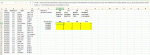
I have a table that I want to summarise a count using certain criteria. That table is in cells F7 to J11.

The data that are being checked are in cells A1 to D24. I want the summary table noted above to check the date (column A), reference number column B), start & end (columns C & D) and only count if the locations found in the Start & End columns are not noted in the "Allowed Locations" which are identified in G1 to J4.

I have manually entered what the values should be in cells G8 to J11.

I have a feeling that it may be a MATCH / INDEX type solution but not sure. If there is an easier way, then all the better.

Thanks

Book1
	A	B	C	D	E	F	G	H	I	J
1	Date	Reference	Start	End		Reference	567	111	234	678
2	1/04/2020	567	Cairo	New York		Allowed Locations	Boston	Cairo	Boston	Auckland
3	1/04/2020	567	Boston	New York			New York	Auckland	New York	Las Vegas
4	1/04/2020	567	Boston	New York			Calgary	New York	Cairo	Los Angeles
5	1/04/2020	111	Dallas	Boston
6	1/04/2020	567	Boston	Calgary
7	2/04/2020	234	Boston	Cairo		Should Read -	567	111	234	678
8	2/04/2020	234	Los Angeles	Boston		1/04/2020	1	1	0	0
9	2/04/2020	567	Boston	Boston		2/04/2020	0	1	1	0
10	2/04/2020	567	Boston	New York		3/04/2020	0	2	0	3
11	2/04/2020	111	Boston	New York		4/04/2020	0	0	2	0
12	2/04/2020	567	Boston	New York
13	3/04/2020	111	New York	New York
14	3/04/2020	111	New York	Los Angeles
15	3/04/2020	111	Las Vegas	New York
16	3/04/2020	678	New York	Cairo
17	3/04/2020	678	New York	Cairo
18	3/04/2020	678	Seattle	Cairo
19	4/04/2020	111	New York	Cairo
20	4/04/2020	111	New York	Cairo
21	4/04/2020	567	New York	Boston
22	4/04/2020	234	Auckland	Boston
23	4/04/2020	234	Cairo	Boston
24	4/04/2020	234	Auckland	Boston
Sheet7

 

[Fluff]

How about

+Fluff New.xlsm
	A	B	C	D	E	F	G	H	I	J
1	Date	Reference	Start	End		Reference	567	111	234	678
2	01/04/2020	567	Cairo	New York		Allowed Locations	Boston	Cairo	Boston	Auckland
3	01/04/2020	567	Boston	New York			New York	Auckland	New York	Las Vegas
4	01/04/2020	567	Boston	New York			Calgary	New York	Cairo	Los Angeles
5	01/04/2020	111	Dallas	Boston
6	01/04/2020	567	Boston	Calgary
7	02/04/2020	234	Boston	Cairo
8	02/04/2020	234	Los Angeles	Boston		01/04/2020	1	1	0	0
9	02/04/2020	567	Boston	Boston		02/04/2020	0	1	1	0
10	02/04/2020	567	Boston	New York		03/04/2020	0	2	0	3
11	02/04/2020	111	Boston	New York		04/04/2020	0	0	2	0
12	02/04/2020	567	Boston	New York
13	03/04/2020	111	New York	New York
14	03/04/2020	111	New York	Los Angeles
15	03/04/2020	111	Las Vegas	New York
16	03/04/2020	678	New York	Cairo
17	03/04/2020	678	New York	Cairo
18	03/04/2020	678	Seattle	Cairo
19	04/04/2020	111	New York	Cairo
20	04/04/2020	111	New York	Cairo
21	04/04/2020	567	New York	Boston
22	04/04/2020	234	Auckland	Boston
23	04/04/2020	234	Cairo	Boston
24	04/04/2020	234	Auckland	Boston
Report

Cell Formulas
Range	Formula
F8:F11	F8	=UNIQUE(A2:A24)
G8:J11	G8	=COUNT(FILTER(ROW($A$2:$A$24),($A$2:$A$24=$F8)*($B$2:$B$24=G$1)*((ISERROR(MATCH($C$2:$C$24,G$2:G$4,0)))+(ISERROR(MATCH($D$2:$D$24,G$2:G$4,0))))))
Dynamic array formulas.

 

[Steve 1962]

Hey thanks Fluff -

I don't have the UNIQUE function in my version of Excel. I might be able to find some way around this.

Is there an equivalent function in earlier versions (2013) ?

Thanks

 

[Steve 1962]

Also don't have FILTER function.

 

[Fluff]

Unfortunately, that was the only way I could find, hopefully somebody else will step in.

 

[Steve 1962]

Hey thanks Fluff - I'll keep advertising for help.

 

[Steve 1962]

Not sure if it helps but I don't need formuals for dates in cells F8 to F11. They will be hard coded in the cells.

 

[Amit Tandon]

Refer enclosed image - Enter below formula as an Array formula (Ctrl+Shift+Enter) in cell G8 and copy to the right and down:

=SUM(--(FREQUENCY(IF(ISNA(MATCH($C$2:$D$24,G$2:G$4,0))*ISNUMBER(MATCH($A$2:$A$24,$F8,0))*ISNUMBER(MATCH($B$2:$B$24,G$1,0)),ROW($A$2:$A$24)-ROW($A$2)+1,""),ROW($A$2:$A$24)-ROW($A$2)+1)>0))

 

[sandy666]

maybe something like this

or

 

[Steve 1962]

It appears from above that it is working however, I seem to getting a different answer my end.

See below -

Book1
	A	B	C	D	E	F	G	H	I	J
1	Date	Reference	Start	End		Reference	567	111	234	678
2	1/04/2020	567	Cairo	New York		Allowed Locations	Boston	Cairo	Boston	Auckland
3	1/04/2020	567	Boston	New York			New York	Auckland	New York	Las Vegas
4	1/04/2020	567	Boston	New York			Calgary	New York	Cairo	Los Angeles
5	1/04/2020	111	Dallas	Boston
6	1/04/2020	567	Boston	Calgary
7	2/04/2020	234	Boston	Cairo		Should Read -	567	111	234	678
8	2/04/2020	234	Los Angeles	Boston		1/04/2020	0	0	0	0
9	2/04/2020	567	Boston	Boston		2/04/2020	0	0	0	0
10	2/04/2020	567	Boston	New York		3/04/2020	0	0	0	0
11	2/04/2020	111	Boston	New York		4/04/2020	0	0	2	0
12	2/04/2020	567	Boston	New York
13	3/04/2020	111	New York	New York
14	3/04/2020	111	New York	Los Angeles
15	3/04/2020	111	Las Vegas	New York
16	3/04/2020	678	New York	Cairo
17	3/04/2020	678	New York	Cairo
18	3/04/2020	678	Seattle	Cairo
19	4/04/2020	111	New York	Cairo
20	4/04/2020	111	New York	Cairo
21	4/04/2020	567	New York	Boston
22	4/04/2020	234	Auckland	Boston
23	4/04/2020	234	Cairo	Boston
24	4/04/2020	234	Auckland	Boston
Mr Excel

Cell Formulas
Range	Formula
G8:J11	G8	{=SUM(--(FREQUENCY(IF(ISNA(MATCH($C$2:$D$24,G$2:G$4,0))*ISNUMBER(MATCH($A$2:$A$24,$F8,0))*ISNUMBER(MATCH($B$2:$B$24,G$1,0)),ROW($A$2:$A$24)-ROW($A$2)+1,""),ROW($A$2:$A$24)-ROW($A$2)+1)>0))}
Press CTRL+SHIFT+ENTER to enter array formulas surrounded with curly braces.