Counting given amount of consecutives

Marvo

Board Regular
Joined
Nov 27, 2023
Messages
155
Office Version
  1. 2021
Platform
  1. Windows
Hi Again, I've constructed a formula

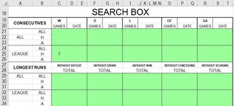
=XLOOKUP("W",K:K,B:B,,0,-1)

That works well, it finds the most recent time there was a "W" in a column.

How could I change that formula so that it would look for a given amount of consecutive "W"s please?

I'm thinking maybe of having it refer to a cell $F$5579 with a number in it, then look for that amount of "W"'s.

So if I put a 3 in the reference cell, the formula would then look for the most recent time there were 3 consecutive "W"'s in column K.

Would that be the way to go?

As always any help appreciated and if there's a better way of achieving the desired result I'm happy to be educated.


/?
 

Excel Facts

How to create a cell-sized chart?
Tiny charts, called Sparklines, were added to Excel 2010. Look for Sparklines on the Insert tab.
Thanks but I dont need the total, I need to find consecutives. As in, when was the last time we won 4 in a row.
 
Upvote 0
us a formula to increment a number for each consecutive W, Then when you go back to 0 use another column to flag that number as the streak.
Assuming I've added 2 columns next to K which contains the W's
L2 =
Excel Formula:
=IF(K2="W",1,0)
L3 =
Excel Formula:
=IF(K3="W",L2+1,0)
M2 =
Excel Formula:
=IF(AND(L3=0,L2<>0),"Streak","")
Then you can filter by Streak.
Or you can set up a table to count the number of times a streak has occurred
# Consecutive wins
1
Excel Formula:
=COUNTIFS(L:L,R1,M:M,"Streak")
:Fill down
2
3
4
5
 
Upvote 0
Thanks. I'll give that a go, I already have a helper column where W=3, D=1 & L=0 so I could use that. I'll report back.

I've found a similar question by jchick90 posted Feb 22nd which has a different method, I might try to cannibalise that too, see which works best.
 
Upvote 0
What should happen if the last long winning streak was actually 5 but you are looking for the last time you won 4 in a row? See my first example below.

A few small varied sets of sample data and expected results with XL2BB would help clarify what you have, what where it is and what you are trying to achieve if the following is not what you want.

Sounds like a helper column would be acceptable. Would a vba solution also be acceptable?

Pending some of the answers above, this could be a possible helper column method.
Note that in this first example the date reported actually ends a streak of 5 but that ends with a streak of 4 by my reckoning. Is that what you want?

24 03 18.xlsm
BKLMNO
1DateResultHelperStreak of interestW/L/D StreakLast time
21/01/2024WW14W20/01/2024
32/01/2024LL1
43/01/2024LL2
54/01/2024WW1
65/01/2024WW2
76/01/2024WW3
87/01/2024WW4
98/01/2024LL1
109/01/2024LL2
1110/01/2024LL3
1211/01/2024WW1
1312/01/2024WW2
1413/01/2024LL1
1514/01/2024LL2
1615/01/2024LL3
1716/01/2024WW1
1817/01/2024WW2
1918/01/2024WW3
2019/01/2024WW4
2120/01/2024WW4
2221/01/2024DD1
2322/01/2024DD2
2423/01/2024WW1
2524/01/2024WW2
2625/01/2024WW3
2726/01/2024LL1
2827/01/2024LL2
2928/01/2024DD1
3029/01/2024LL1
3130/01/2024LL2
32 
33 
Streak
Cell Formulas
RangeFormula
O2O2=XLOOKUP(N2&M2,L2:L40,B2:B40,"N/A",,-1)
L2:L33L2=IF(K2="","",K2&IF(K1=K2,MIN(MID(L1,2,9)+1,M$2),1))


A couple of other examples.

24 03 18.xlsm
BKLMNO
1DateResultHelperStreak of interestW/L/D StreakLast time
21/01/2024WW14LN/A
32/01/2024LL1
43/01/2024LL2
54/01/2024WW1
65/01/2024WW2
76/01/2024WW3
87/01/2024WW4
98/01/2024LL1
109/01/2024LL2
1110/01/2024LL3
1211/01/2024WW1
1312/01/2024WW2
1413/01/2024LL1
1514/01/2024LL2
1615/01/2024LL3
1716/01/2024WW1
1817/01/2024WW2
1918/01/2024WW3
2019/01/2024WW4
2120/01/2024WW4
2221/01/2024DD1
2322/01/2024DD2
2423/01/2024WW1
2524/01/2024WW2
2625/01/2024WW3
2726/01/2024LL1
2827/01/2024LL2
2928/01/2024DD1
3029/01/2024LL1
3130/01/2024LL2
32 
Streak (2)
Cell Formulas
RangeFormula
O2O2=XLOOKUP(N2&M2,L2:L40,B2:B40,"N/A",,-1)
L2:L32L2=IF(K2="","",K2&IF(K1=K2,MIN(MID(L1,2,9)+1,M$2),1))


24 03 18.xlsm
BKLMNO
1DateResultHelperStreak of interestW/L/D StreakLast time
21/01/2024WW12D22/01/2024
32/01/2024LL1
43/01/2024LL2
54/01/2024WW1
65/01/2024WW2
76/01/2024WW2
87/01/2024WW2
98/01/2024LL1
109/01/2024LL2
1110/01/2024LL2
1211/01/2024WW1
1312/01/2024WW2
1413/01/2024LL1
1514/01/2024LL2
1615/01/2024LL2
1716/01/2024WW1
1817/01/2024WW2
1918/01/2024WW2
2019/01/2024WW2
2120/01/2024WW2
2221/01/2024DD1
2322/01/2024DD2
2423/01/2024WW1
2524/01/2024WW2
2625/01/2024WW2
2726/01/2024LL1
2827/01/2024LL2
2928/01/2024DD1
3029/01/2024LL1
3130/01/2024LL2
32 
Streak (3)
Cell Formulas
RangeFormula
O2O2=XLOOKUP(N2&M2,L2:L40,B2:B40,"N/A",,-1)
L2:L32L2=IF(K2="","",K2&IF(K1=K2,MIN(MID(L1,2,9)+1,M$2),1))
 
Upvote 0
I think VBA would be best, I've just started learning that. It seems to work through searches much quicker. Only know the basics though. Managed to do some sorts.

I've still got a lot to work through, will need criteria added to further searches. I cant get that XL2BB to work but I can upload the workbook to the cloud for sharing.

I usually ask one question, then try to apply the answer to several others.

Sorry for the tardy response, been incredibly busy this morning.
 
Upvote 0
Just to clarify, the question is, if a team was to draw their last 5 matches, when was the last time that happened? That could go back several years, even decades.

The criteria to be added would be is the game either a league game or all matches including cups.

Then a further criteria would be either home or away.
 
Upvote 0
So this is the search box I will be using. The plan is, I put a figure in one of the cells, in the image its a 7 in C25.
The formula or VBA would then be searching for the most recent time the team "W" (won) in C19, 7 C25, consecutive "H" (home) in B25, "LEAGUE" in A25 games.
The search for the "W" is on worksheet "ALL" column K.
The search for "League" is on worksheet "ALL" column J.
The search for the "H" is on worksheet "ALL" column E.

Each column is currently 5558 rows long.

Would it help if I shared the workbook on one drive?
 

Attachments

  • Mr Excel.JPG
    Mr Excel.JPG
    64.4 KB · Views: 5
Upvote 0
Sorry, the result would be the date (worksheet ALL Column B) to be entered in D25 with a hyperlink to the actual sequence.

This would only be required on a few occasions during the season so an update button would be much better than formula continually searching.
 
Upvote 0

Forum statistics

Threads
1,215,073
Messages
6,122,970
Members
449,095
Latest member
Mr Hughes

We've detected that you are using an adblocker.

We have a great community of people providing Excel help here, but the hosting costs are enormous. You can help keep this site running by allowing ads on MrExcel.com.
Allow Ads at MrExcel

Which adblocker are you using?

Disable AdBlock

Follow these easy steps to disable AdBlock

1)Click on the icon in the browser’s toolbar.
2)Click on the icon in the browser’s toolbar.
2)Click on the "Pause on this site" option.
Go back

Disable AdBlock Plus

Follow these easy steps to disable AdBlock Plus

1)Click on the icon in the browser’s toolbar.
2)Click on the toggle to disable it for "mrexcel.com".
Go back

Disable uBlock Origin

Follow these easy steps to disable uBlock Origin

1)Click on the icon in the browser’s toolbar.
2)Click on the "Power" button.
3)Click on the "Refresh" button.
Go back

Disable uBlock

Follow these easy steps to disable uBlock

1)Click on the icon in the browser’s toolbar.
2)Click on the "Power" button.
3)Click on the "Refresh" button.
Go back
Back
Top