Counting Value with Multiple Duplicate Entries?

[privxls]

Hello,

It has been a while since I've been here on the community, I've had some challenges with life and now I seem to be back on track and I hope everyone here are doing fine and well! I wanted to ask a questions regarding a problem that I am currently facing, I have a sheet where it has multiple duplicates.

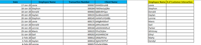
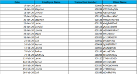
I want to count the sort a list that contains duplicates. Now, while I understand that you may say just remove the duplicates, it is a bit tricky as I am not allowed to remove any duplicates. Let me provide you a bit of information about this: The sheet contains list of employees that have processed transactions for customers. I need to get the exact number that the employee has processed a transaction for each customer. The list contains more than 10K data and it's a combination of unique and duplicates. The reason for duplicates is that some customers are repeat customers and they use the same transaction number. See screenshot below:

I want to get each employee's number of interactions per customer. Also, I want to get each employee's number of interactions per customer excluding duplicates.

I've been playing around =COUNTIFS function and searched all over but can't seem to get an answer.

Hoping someone can help me

Thank you.

 

[privxls]

Here's a mini-sheet for anyone's reference:

count-dummy file.xlsx
	A	B	C	D	E	F	G	H
1	Date	Employee Name	Transaction Number	Client Name			Employee Name	# of Customer Interaction
2	17-Jan-20	Lexie	500087	KHH05tnzAB			Lexie
3	18-Jan-20	Stephon	500284	YWENe1qQRe			Stephon
4	18-Jan-20	Donald	600083	4jB8VBYQyx			Donald
5	20-Jan-20	Kaylan	500155	Gw8AccokMC			Kaylan
6	20-Jan-20	Stephon	600145	mHWFoYGHBb			Lonnie
7	21-Jan-20	Lexie	600171	eMgBrH50wF			Mavis
8	22-Jan-20	Donald	500156	yMKo34zeH9			Gail
9	26-Jan-20	Lonnie	600184	uGGSkWARwZ			Parker
10	29-Jan-20	Mavis	500225	lYhsZ3Ij6w			Whitney
11	31-Jan-20	Gail	600202	jH1tX49GCW			Ethyl
12	2-Feb-20	Gail	500012	19S6zPkYsz			Marty
13	3-Feb-20	Kaylan	600014	7gW1TDTfVf			Kendyl
14	4-Feb-20	Lonnie	500057	yfwNJ1P64x
15	7-Feb-20	Parker	500159	sKcsa879Pa
16	7-Feb-20	Whitney	500288	4ECUDhRGxy
17	11-Feb-20	Lexie	500120	57H88zSO2D
18	14-Feb-20	Kaylan	500039	UNxEeht4S1
19	14-Feb-20	Mavis	600252	POUQaOmkIa
20	19-Feb-20	Lonnie	500199	uT36HiDcZp
21	26-Feb-20	Gail	500249	rtOs44cSWo
22	26-Feb-20	Stephon	500018	FOuBf0V7nM
23	28-Feb-20	Ethyl	500046	xe3AARCZnk
24	2-Mar-20	Parker	500000	NAxJ66g8Gl
25	3-Mar-20	Gail	500110	UNxEeht4S1
26	6-Mar-20	Marty	500295	CoD8PpkZZI
27	8-Mar-20	Stephon	500298	KjQHSxNxzB
28	13-Mar-20	Kaylan	600033	0IyXhlLBzO
29	17-Mar-20	Marty	500062	35HGj0R46Z
30	18-Mar-20	Marty	500214	8kUptBJuzx
31	18-Mar-20	Mavis	500106	mErxoNMT8K
32	18-Mar-20	Kaylan	600042	JD4OZJxpeW
33	22-Mar-20	Gail	500213	sp4ifBWNFY
34	22-Mar-20	Kendyl	600170	Ijo3W57IHH
35	26-Mar-20	Donald	500034	24o1xaHseA
36	28-Mar-20	Donald	600215	fPJKZnlBVc
37	29-Mar-20	Mavis	600159	UDYODC92oR
38	30-Mar-20	Stephon	500202	mpPp98ssPE
39	5-Apr-20	Lexie	500160	RXVJ8uyUFt
40	6-Apr-20	Marty	500232	A4e7EYwGP5
41	7-Apr-20	Mavis	500263	iYfVd24etp
42	9-Apr-20	Kendyl	600035	kn1d7XbKRQ
43	13-Apr-20	Lexie	500189	feMpBeoLbn
44	13-Apr-20	Stephon	500114	rJa0GkF7Ej
45	16-Apr-20	Mavis	500268	D0nOXA0Khw
46	16-Apr-20	Mavis	500131	dPcdGzquKR
47	18-Apr-20	Donald	600125	bPfqP4Sl6I
48	19-Apr-20	Kendyl	600113	yKqY2YeJxf
49	20-Apr-20	Lexie	500037	U4h52Y07R5
50	23-Apr-20	Whitney	500233	yfwNJ1P64x
Sheet1

 

[Peter_SSs]

I suggest that you update your Account details (or click your user name at the top right of the forum) so helpers always know what Excel version(s) & platform(s) you are using as the best solution often varies by version. (Don’t forget to scroll down & ‘Save’)

Your question may also be clearer if you include the expected results for that sample data in column H (& for the second question in column I) and post the mini sheet again with any further explanation about how those expected results were obtained manually.

Note too that you can resize the columns to help the mini sheet fit better in your forum post.

 

[mohadin]

Employee Name	# of Customer Interaction
Lexie	6
Stephon	6
Donald	5
Kaylan	5
Lonnie	3
Mavis	7
Gail	5
Parker	2
Whitney	2
Ethyl	1
Marty	4
Kendyl	3

If the expected result like above

Sub test()
    Dim a
    Dim i&
    a = Sheet1.Range("B2:B" & Sheet1.Cells(Rows.Count, 2).End(xlUp).Row)
    With CreateObject("scripting.dictionary")
        For i = 1 To UBound(a)
            If a(i, 1) <> 0 Then
                If Not .exists(a(i, 1)) Then
                    .Add a(i, 1), 1
                Else
                    .Item(a(i, 1)) = .Item(a(i, 1)) + 1
                End If
            End If
        Next
             Sheets("Sheet1").Cells(2, 7).Resize(.Count, 2) = Application.Transpose(Application.Index(Array(.keys, .items), 0, 0))
    End With
End Sub

 

[privxls]

Employee Name	# of Customer Interaction
Lexie	6
Stephon	6
Donald	5
Kaylan	5
Lonnie	3
Mavis	7
Gail	5
Parker	2
Whitney	2
Ethyl	1
Marty	4
Kendyl	3

If the expected result like above

Sub test()
    Dim a
    Dim i&
    a = Sheet1.Range("B2:B" & Sheet1.Cells(Rows.Count, 2).End(xlUp).Row)
    With CreateObject("scripting.dictionary")
        For i = 1 To UBound(a)
            If a(i, 1) <> 0 Then
                If Not .exists(a(i, 1)) Then
                    .Add a(i, 1), 1
                Else
                    .Item(a(i, 1)) = .Item(a(i, 1)) + 1
                End If
            End If
        Next
             Sheets("Sheet1").Cells(2, 7).Resize(.Count, 2) = Application.Transpose(Application.Index(Array(.keys, .items), 0, 0))
    End With
End Sub

Thank you Mohadin. Can you please help me understand how the code works?

 

[Fluff]

@privxls maybe you missed Peter's post. This can easily be done with a formula depending on your version of Excel

 

[privxls]

@Fluff Thanks for pointing it out. I've added my version and platform now.

I appreciate the mods for always helping out @Peter_SSs

 

[Fluff]

Thanks for that, how about

Fluff.xlsm
	A	B	C	D	E	F	G	H
1	Date	Employee Name	Transaction Number	Client Name			Employee Name	# of Customer Interaction
2	17/01/2020	Lexie	500087	KHH05tnzAB			Lexie	6
3	18/01/2020	Stephon	500284	YWENe1qQRe			Stephon	6
4	18/01/2020	Donald	600083	4jB8VBYQyx			Donald	5
5	20/01/2020	Kaylan	500155	Gw8AccokMC			Kaylan	5
6	20/01/2020	Stephon	600145	mHWFoYGHBb			Lonnie	3
7	21/01/2020	Lexie	600171	eMgBrH50wF			Mavis	7
8	22/01/2020	Donald	500156	yMKo34zeH9			Gail	5
9	26/01/2020	Lonnie	600184	uGGSkWARwZ			Parker	2
10	29/01/2020	Mavis	500225	lYhsZ3Ij6w			Whitney	2
11	31/01/2020	Gail	600202	jH1tX49GCW			Ethyl	1
12	02/02/2020	Gail	500012	19S6zPkYsz			Marty	4
13	03/02/2020	Kaylan	600014	7gW1TDTfVf			Kendyl	3
14	04/02/2020	Lonnie	500057	yfwNJ1P64x
15	07/02/2020	Parker	500159	sKcsa879Pa
16	07/02/2020	Whitney	500288	4ECUDhRGxy
17	11/02/2020	Lexie	500120	57H88zSO2D
18	14/02/2020	Kaylan	500039	UNxEeht4S1
19	14/02/2020	Mavis	600252	POUQaOmkIa
20	19/02/2020	Lonnie	500199	uT36HiDcZp
21	26/02/2020	Gail	500249	rtOs44cSWo
22	26/02/2020	Stephon	500018	FOuBf0V7nM
23	28/02/2020	Ethyl	500046	xe3AARCZnk
24	02/03/2020	Parker	500000	NAxJ66g8Gl
25	03/03/2020	Gail	500110	UNxEeht4S1
26	06/03/2020	Marty	500295	CoD8PpkZZI
27	08/03/2020	Stephon	500298	KjQHSxNxzB
28	13/03/2020	Kaylan	600033	0IyXhlLBzO
29	17/03/2020	Marty	500062	35HGj0R46Z
30	18/03/2020	Marty	500214	8kUptBJuzx
31	18/03/2020	Mavis	500106	mErxoNMT8K
32	18/03/2020	Kaylan	600042	JD4OZJxpeW
33	22/03/2020	Gail	500213	sp4ifBWNFY
34	22/03/2020	Kendyl	600170	Ijo3W57IHH
35	26/03/2020	Donald	500034	24o1xaHseA
36	28/03/2020	Donald	600215	fPJKZnlBVc
37	29/03/2020	Mavis	600159	UDYODC92oR
38	30/03/2020	Stephon	500202	mpPp98ssPE
39	05/04/2020	Lexie	500160	RXVJ8uyUFt
40	06/04/2020	Marty	500232	A4e7EYwGP5
41	07/04/2020	Mavis	500263	iYfVd24etp
42	09/04/2020	Kendyl	600035	kn1d7XbKRQ
43	13/04/2020	Lexie	500189	feMpBeoLbn
44	13/04/2020	Stephon	500114	rJa0GkF7Ej
45	16/04/2020	Mavis	500268	D0nOXA0Khw
46	16/04/2020	Mavis	500131	dPcdGzquKR
47	18/04/2020	Donald	600125	bPfqP4Sl6I
48	19/04/2020	Kendyl	600113	yKqY2YeJxf
49	20/04/2020	Lexie	500037	U4h52Y07R5
50	23/04/2020	Whitney	500233	yfwNJ1P64x
Main

Cell Formulas
Range	Formula
G2:G13	G2	=UNIQUE(FILTER(B2:B1000,B2:B1000<>""))
H2:H13	H2	=ROWS(UNIQUE(FILTER(D2:D1000,B2:B1000=G2)))
Dynamic array formulas.

 

[privxls]

Thanks for that, how about

Fluff.xlsm
	A	B	C	D	E	F	G	H
1	Date	Employee Name	Transaction Number	Client Name			Employee Name	# of Customer Interaction
2	17/01/2020	Lexie	500087	KHH05tnzAB			Lexie	6
3	18/01/2020	Stephon	500284	YWENe1qQRe			Stephon	6
4	18/01/2020	Donald	600083	4jB8VBYQyx			Donald	5
5	20/01/2020	Kaylan	500155	Gw8AccokMC			Kaylan	5
6	20/01/2020	Stephon	600145	mHWFoYGHBb			Lonnie	3
7	21/01/2020	Lexie	600171	eMgBrH50wF			Mavis	7
8	22/01/2020	Donald	500156	yMKo34zeH9			Gail	5
9	26/01/2020	Lonnie	600184	uGGSkWARwZ			Parker	2
10	29/01/2020	Mavis	500225	lYhsZ3Ij6w			Whitney	2
11	31/01/2020	Gail	600202	jH1tX49GCW			Ethyl	1
12	02/02/2020	Gail	500012	19S6zPkYsz			Marty	4
13	03/02/2020	Kaylan	600014	7gW1TDTfVf			Kendyl	3
14	04/02/2020	Lonnie	500057	yfwNJ1P64x
15	07/02/2020	Parker	500159	sKcsa879Pa
16	07/02/2020	Whitney	500288	4ECUDhRGxy
17	11/02/2020	Lexie	500120	57H88zSO2D
18	14/02/2020	Kaylan	500039	UNxEeht4S1
19	14/02/2020	Mavis	600252	POUQaOmkIa
20	19/02/2020	Lonnie	500199	uT36HiDcZp
21	26/02/2020	Gail	500249	rtOs44cSWo
22	26/02/2020	Stephon	500018	FOuBf0V7nM
23	28/02/2020	Ethyl	500046	xe3AARCZnk
24	02/03/2020	Parker	500000	NAxJ66g8Gl
25	03/03/2020	Gail	500110	UNxEeht4S1
26	06/03/2020	Marty	500295	CoD8PpkZZI
27	08/03/2020	Stephon	500298	KjQHSxNxzB
28	13/03/2020	Kaylan	600033	0IyXhlLBzO
29	17/03/2020	Marty	500062	35HGj0R46Z
30	18/03/2020	Marty	500214	8kUptBJuzx
31	18/03/2020	Mavis	500106	mErxoNMT8K
32	18/03/2020	Kaylan	600042	JD4OZJxpeW
33	22/03/2020	Gail	500213	sp4ifBWNFY
34	22/03/2020	Kendyl	600170	Ijo3W57IHH
35	26/03/2020	Donald	500034	24o1xaHseA
36	28/03/2020	Donald	600215	fPJKZnlBVc
37	29/03/2020	Mavis	600159	UDYODC92oR
38	30/03/2020	Stephon	500202	mpPp98ssPE
39	05/04/2020	Lexie	500160	RXVJ8uyUFt
40	06/04/2020	Marty	500232	A4e7EYwGP5
41	07/04/2020	Mavis	500263	iYfVd24etp
42	09/04/2020	Kendyl	600035	kn1d7XbKRQ
43	13/04/2020	Lexie	500189	feMpBeoLbn
44	13/04/2020	Stephon	500114	rJa0GkF7Ej
45	16/04/2020	Mavis	500268	D0nOXA0Khw
46	16/04/2020	Mavis	500131	dPcdGzquKR
47	18/04/2020	Donald	600125	bPfqP4Sl6I
48	19/04/2020	Kendyl	600113	yKqY2YeJxf
49	20/04/2020	Lexie	500037	U4h52Y07R5
50	23/04/2020	Whitney	500233	yfwNJ1P64x
Main

Cell Formulas
Range	Formula
G2:G13	G2	=UNIQUE(FILTER(B2:B1000,B2:B1000<>""))
H2:H13	H2	=ROWS(UNIQUE(FILTER(D2:D1000,B2:B1000=G2)))
Dynamic array formulas.

Hey @Fluff ,

You're a life saver, the formula worked as intended!

I'll make note of this formula from now on

By the way, is it okay to ask for additional information from you? I wanted to ask how the formula works? These are the only ones that I understand thus far:

=UNIQUE - provides Unique values on selected column

However, I don't seem to understand the use of =FILTER and the operator "<>", what does B2:B1000 use the "<>" for?. I've tried just using =FILTER and it just lists the exact data from the selected column. So I'm not quite understand the need to do it. Why can I just not use the =UNIQUE function alone?

Also, for =ROWS, what is the need to add it in the formula?

I really appreciate your very kind help <3

 

[Fluff]

The filter is there to remove empty rows so that you don't need to use the exact range of your data.