Jane_Hogan
New Member
- Joined
- Sep 20, 2023
- Messages
- 5
- Office Version
- 365
- Platform
- Windows
Hi all,
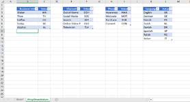
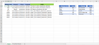
I have created several dropdown lists on a worksheet which all need to display different values in order to provide input for a name generator cell (using the textjoin formula). I found a VBA code which let's me display different values in a dropdown list ; For example sheet1 shows a dropdown list in column B with the option water which displays as 'WA' and Thee as 'TH' and so on. I would like to apply the same to the dropdown lists in column C to E but I'm unable to solve 2 problems:
1) The VBA code only works with the active sheet (=Sheet1). What code should I use to reference the other sheet (=DropDownValues)? I prefer to keep the dropdown values on a separate sheet so it can be hidden.
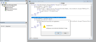
2) Sheet1 has several dropdown lists (column B to E) which need to display different values coming from different tables/cells. I tried to use the same VBA code for the other dropdown values on the active sheet but it's not working and I'm seeing a compile error (see screenshots)). How can I apply similar VBA codes in one project/sheet?
Thank you for your help!
Thank you for your help!
I have created several dropdown lists on a worksheet which all need to display different values in order to provide input for a name generator cell (using the textjoin formula). I found a VBA code which let's me display different values in a dropdown list ; For example sheet1 shows a dropdown list in column B with the option water which displays as 'WA' and Thee as 'TH' and so on. I would like to apply the same to the dropdown lists in column C to E but I'm unable to solve 2 problems:
1) The VBA code only works with the active sheet (=Sheet1). What code should I use to reference the other sheet (=DropDownValues)? I prefer to keep the dropdown values on a separate sheet so it can be hidden.
2) Sheet1 has several dropdown lists (column B to E) which need to display different values coming from different tables/cells. I tried to use the same VBA code for the other dropdown values on the active sheet but it's not working and I'm seeing a compile error (see screenshots)). How can I apply similar VBA codes in one project/sheet?
Thank you for your help!
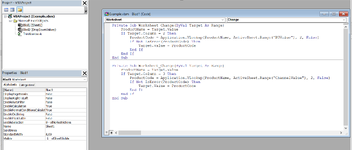
VBA Code:
Private Sub Worksheet_Change(ByVal Target As Range)

ProductName = Target.Value

If Target.Column = 2 Then

ProductCode = Application.VLookup(ProductName, ActiveSheet.Range("BUValue"), 2, False)

If Not IsError(ProductCode) Then

Target.Value = ProductCode

End If

End If

End Sub
Thank you for your help!
") . So, I'm just guessing here. This is how you can implement one event trigger for more than one column
. So, I'm just guessing here. This is how you can implement one event trigger for more than one column


