Criteria >=""

[broth]

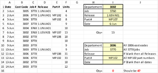
I have a formula that is supposed to return a value in one column based on multiple criteria in multiple columns. One of the criteria is that if the criteria cell is blank ("") or the word "ALL" is selected then the criteria for the column will be blank or not blank. The other criteria option is a specific match. How do you specify that the criteria includes everything or a specific value?
Formula in I16 = =SUMIFS($G$3:$G$16,$B$3:$B$16,IF(OR(J15="",J15="ALL"),">="&"",J15),$C$3:$C$16,IF(OR(J11="",J11="ALL"),">="&"",J11),$D$3:$D$16,IF(OR(J12="",J12="ALL"),">="&"",J12),$E$3:$E$16,IF(OR(J13="",J13="ALL"),">="&"",J13),$F$3:$F$16,IF(OR(J14="",J14="ALL"),">="&"",J14))

 

[Eric W]

SUMIFS can be quite finicky about what parameters you use, especially between numeric and non-numeric data. I expect that the problem is how you set up the parameters you used for the ALL cases, like ">="&"". Instead of that, try "<>.1" where the .1 is a value that will never exist in any column. This should work for both numeric and non-numeric values. For example:

Book1
	A	B	C	D	E	F	G	H	I
1	Date	Cost Code	Job #	Release	Part #	Units		Department	3002
2	1-Jun	3005	3770	1.UNVA01		4		Job	3760
3	2-Jun	3006	3770	1.UNVA01	MP102	6		Release	1.USVA01
4	3-Jun	3006	3770		MP102	8		Part #	MP107
5	4-Jun	3007	3770	1.UNVA01		9		Date	6-Jun
6	5-Jun	3004	3760	1.UNVA01		10
7	6-Jun	3002	3760	1.USVA01	MP107	13		Qty=	13
8	7-Jun	3002	3770		MP108	10
9	8-Jun	3002	3770			10
10	9-Jun	3003	3770			9		Department	3006
11	10-Jun	3003	3770	1.UNVA01		9		Job	3770
12	11-Jun	3006	3770		MP108	31		Release
13	12-Jun	3006	3770		MP102	33		Part #	MP102
14	13-Jun	3002	3770			10		Date
15	14-Jun	3003	3770			12
16								Qty=	47
Sheet1

Cell Formulas
Range	Formula
I7,I16	I7	=LET(p,IF((I1:I5="")+(I1:I5="ALL"),"<>.1",I1:I5),SUMIFS(F:F,A:A,INDEX(p,5),B:B,INDEX(p,1),C:C,INDEX(p,2),D:D,INDEX(p,3),E:E,INDEX(p,4)))

2 quick suggestions to help you get more and faster responses. Using XL2BB makes it easier for the helpers here to work on your problem. Also, please update your profile to show what version of Excel you're using. I used LET in my example, but I don't know if it will work for you. If not, try using "<>.1" in your current formula. Good luck!

 

[Tetra201]

Another approach:

=SUMPRODUCT(SUMIFS($G$3:$G$16,
$B$3:$B$16,IF(OR(J15={"","ALL"}),">="&MIN($B$3:$B$16),J15),
$C$3:$C$16,IF(OR(J11={"","ALL"}),">="&MIN($C$3:$C$16),J11),
$D$3:$D$16,IF(OR(J12={"","ALL"}),">="&MIN($D$3:$D$16),J12),
$E$3:$E$16,IF(OR(J13={"","ALL"}),{"","*"},J13),
$F$3:$F$16,IF(OR(J14={"","ALL"}),{"";"*"},J14)))

 

[broth]

SUMIFS can be quite finicky about what parameters you use, especially between numeric and non-numeric data. I expect that the problem is how you set up the parameters you used for the ALL cases, like ">="&"". Instead of that, try "<>.1" where the .1 is a value that will never exist in any column. This should work for both numeric and non-numeric values. For example:

Book1
	A	B	C	D	E	F	G	H	I
1	Date	Cost Code	Job #	Release	Part #	Units		Department	3002
2	1-Jun	3005	3770	1.UNVA01		4		Job	3760
3	2-Jun	3006	3770	1.UNVA01	MP102	6		Release	1.USVA01
4	3-Jun	3006	3770		MP102	8		Part #	MP107
5	4-Jun	3007	3770	1.UNVA01		9		Date	6-Jun
6	5-Jun	3004	3760	1.UNVA01		10
7	6-Jun	3002	3760	1.USVA01	MP107	13		Qty=	13
8	7-Jun	3002	3770		MP108	10
9	8-Jun	3002	3770			10
10	9-Jun	3003	3770			9		Department	3006
11	10-Jun	3003	3770	1.UNVA01		9		Job	3770
12	11-Jun	3006	3770		MP108	31		Release
13	12-Jun	3006	3770		MP102	33		Part #	MP102
14	13-Jun	3002	3770			10		Date
15	14-Jun	3003	3770			12
16								Qty=	47
Sheet1

Cell Formulas
Range	Formula
I7,I16	I7	=LET(p,IF((I1:I5="")+(I1:I5="ALL"),"<>.1",I1:I5),SUMIFS(F:F,A:A,INDEX(p,5),B:B,INDEX(p,1),C:C,INDEX(p,2),D:D,INDEX(p,3),E:E,INDEX(p,4)))

2 quick suggestions to help you get more and faster responses. Using XL2BB makes it easier for the helpers here to work on your problem. Also, please update your profile to show what version of Excel you're using. I used LET in my example, but I don't know if it will work for you. If not, try using "<>.1" in your current formula. Good luck!

I tried your

SUMIFS can be quite finicky about what parameters you use, especially between numeric and non-numeric data. I expect that the problem is how you set up the parameters you used for the ALL cases, like ">="&"". Instead of that, try "<>.1" where the .1 is a value that will never exist in any column. This should work for both numeric and non-numeric values. For example:

Book1
	A	B	C	D	E	F	G	H	I
1	Date	Cost Code	Job #	Release	Part #	Units		Department	3002
2	1-Jun	3005	3770	1.UNVA01		4		Job	3760
3	2-Jun	3006	3770	1.UNVA01	MP102	6		Release	1.USVA01
4	3-Jun	3006	3770		MP102	8		Part #	MP107
5	4-Jun	3007	3770	1.UNVA01		9		Date	6-Jun
6	5-Jun	3004	3760	1.UNVA01		10
7	6-Jun	3002	3760	1.USVA01	MP107	13		Qty=	13
8	7-Jun	3002	3770		MP108	10
9	8-Jun	3002	3770			10
10	9-Jun	3003	3770			9		Department	3006
11	10-Jun	3003	3770	1.UNVA01		9		Job	3770
12	11-Jun	3006	3770		MP108	31		Release
13	12-Jun	3006	3770		MP102	33		Part #	MP102
14	13-Jun	3002	3770			10		Date
15	14-Jun	3003	3770			12
16								Qty=	47
Sheet1

Cell Formulas
Range	Formula
I7,I16	I7	=LET(p,IF((I1:I5="")+(I1:I5="ALL"),"<>.1",I1:I5),SUMIFS(F:F,A:A,INDEX(p,5),B:B,INDEX(p,1),C:C,INDEX(p,2),D:D,INDEX(p,3),E:E,INDEX(p,4)))

2 quick suggestions to help you get more and faster responses. Using XL2BB makes it easier for the helpers here to work on your problem. Also, please update your profile to show what version of Excel you're using. I used LET in my example, but I don't know if it will work for you. If not, try using "<>.1" in your current formula. Good luck!

I used "<>"&.1 and it worked. Thanks.

 

[Eric W]

Glad we could help, and thank you for updating your profile.